*A nonparametrics R project studying the influence of people’s education level on their occupation with the same dataset can be found here: Nonparametric-Statistic-Project

ML-NaiveBayesClassifier

a classification program with Naive Bayes Classifier

Background

This is a classification program implemented with Naive Bayes Classifier.

Training Data: A training set of 1500 census data. Each line of data has 13 features, 5 of which are continuous. The response variables are the salaries of citizens, either >50K or <=50K, based on various features in the data.

Goal: To predict the results of another set of data, given all 13 features of each data.

Language: Java

First 20 Lines of Training Data:

60 Self-emp-not-inc HS-grad 9 Married-civ-spouse Exec-managerial Husband White Male 0 0 50 United-States >50K 
28 Private 9th 4 Never-married Other-service Own-child White Female 0 0 35 El-Salvador <=50K 
46 Private HS-grad 9 Married-spouse-absent Craft-repair Not-in-family White Male 0 0 40 Poland <=50K 
46 Local-gov Some-college 10 Divorced Exec-managerial Not-in-family White Male 0 0 50 United-States <=50K 
37 Private HS-grad 9 Never-married Machine-op-inspct Own-child White Male 0 0 40 United-States <=50K 
28 Private Some-college 10 Married-civ-spouse Sales Wife White Female 0 0 40 United-States >50K 
46 Local-gov Some-college 10 Married-civ-spouse Protective-serv Husband White Male 0 0 40 United-States >50K 
21 Private HS-grad 9 Never-married Machine-op-inspct Own-child White Male 0 0 40 United-States <=50K 
52 Private Bachelors 13 Married-civ-spouse Exec-managerial Husband White Male 15024 0 45 United-States >50K 
52 Private Bachelors 13 Married-civ-spouse Exec-managerial Husband White Male 0 0 40 United-States >50K 
46 Private HS-grad 9 Married-civ-spouse Craft-repair Husband White Male 0 0 40 United-States <=50K 
46 Self-emp-not-inc Bachelors 13 Divorced Craft-repair Not-in-family White Male 0 0 40 United-States <=50K 
28 Private HS-grad 9 Married-civ-spouse Craft-repair Husband White Male 0 0 45 United-States >50K 
60 Private 10th 7 Widowed Machine-op-inspct Unmarried Black Female 0 0 40 United-States <=50K 
33 Private Bachelors 13 Never-married Prof-specialty Own-child White Female 0 0 16 United-States <=50K 
52 Private HS-grad 9 Married-civ-spouse Tech-support Husband White Male 0 0 40 United-States >50K 
28 Private HS-grad 9 Married-civ-spouse Sales Husband White Male 0 0 40 United-States <=50K 
37 Private Bachelors 13 Married-civ-spouse Prof-specialty Husband Amer-Indian-Eskimo Male 0 0 70 United-States >50K 
33 Local-gov HS-grad 9 Married-civ-spouse Protective-serv Husband White Male 0 0 45 United-States <=50K 
21 Private 11th 7 Never-married Sales Own-child White Female 0 0 16 United-States <=50K 

Naive Bayes Classifier

Naive Bayes Classifier uses a simple 2-layer Bayesian Network (1 root node with a layer of leaf nodes).

Learning Process: The learning process pre-calculates all the probabilities of each feature given a response.

Predicting Process: Using the probabilities calculated from the previous step to calculate the probabilities of each response given some features.

There are 2 kinds of data in the training set, continuous and discrete (categorical). Both learning and predicting approaches to these two cases are slightly different, but the overall ideas are similar.

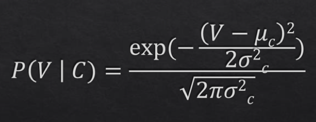
Continuous Case: We need to pre-calculate means and variances for each feature. Then, we use the probability density function showing below to calculate the probabilities, plugging in same Vs for both responses, and choose the higher response as our final prediction.

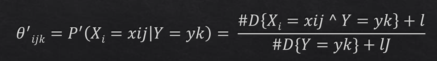
Discrete Case: We need to count occurences of each feature given each response, and calculate the probabilities of each response given a feature. Then, we simply use the Bayes' Law, adding 2 "smoothing factors" as following, to calculate the probabilities for each features. Multiply all the probabilities given both responses, and choose the higher response as our final prediction.

Pseudo Code for Learning

public void readTrainFile(String filename) {

  // READING IN EACH LINE OF THE DATA

  initialize scanners and variables
  // we want 0.7 of the data as training set
  while (hasNextLine) {
    // 70% of the data will be added to training set, the rest will be added to test set
    // TODO change this number to 1 to read all data
    if (Math.random() <= 0.7) { 
      read in the line and add to trainSet
      split the line with whitespace
      if response is '>50K' {
        increment total count of '>50K'
        for each feature
          if numerical value
            take sum
          if discrete value
            increment the count of such aspect of such feature
      } else if response is '<=50K' 
        do the same for response '<=50K'
    } else
      skip and add the line to test set
  }

  // PROCESS DATA

  // initialize smoothing factors
  double l = 1.0;
  double j = 0.0;
  calculate proportion of each aspects using: (D(x&y)+l) / (D(y)+lj)
  add up total count 
  calculate proportions of each response
  calculate means and variances of continuous features of each response
}

Pseudo Code for Predicting

public void makePredictions(String testDataFilepath) {
  initialize scanner and variables

  while (hasNextLine) {
    read in and split the line with whitespace
    for each feature
      if numerical value 
        multiply probabilities of each response using probability density function
      else 
        multiply probabilities of each response using Bayes Law
  }
  print the response with higher probability
}

Testing

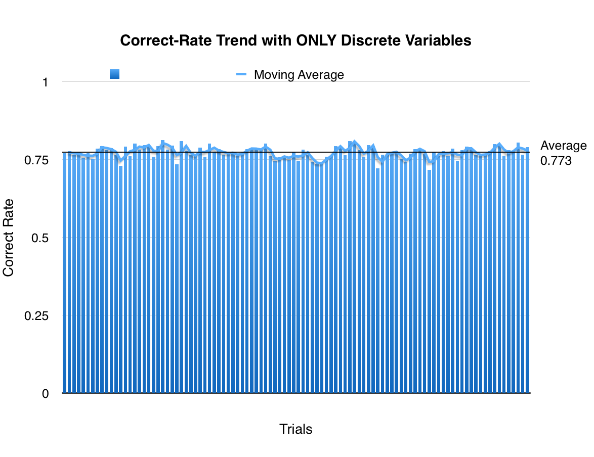
To test the efficiency of the algorithm, I first only implemented the discrete cases, and use 0.7 of the data as training set and the other 0.3 as test set. Applying only discrete rules, and have the algorithm run 100 times with random 0.7 of the data as training set, we get an average of 0.773 correction rate:

Then I implemented the continuous cases and combined the probability functions with the discrete cases.

Analysis

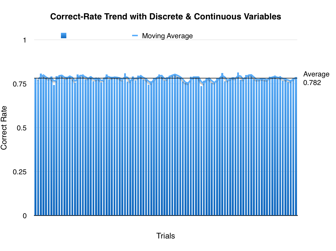
Not surprisingly, the algorithm with continuous taken into consideration is more effective than the one without. Our original algorithm has an average of 0.773 correction rate of 100 random trials, whereas the new algorithm has 0.782 on average. There is a 0.009 of improvement on correct rate. The improvement is not too significant.

The testing results we saw throughout this project demonstrated that this algorithm rely mostly on discrete variables than continuous variables. One of the reasons could be that some of the continuous variables are all 0s. Please inspect the Sample Data.

Overall, this project demonstrated that NaiveBayes algorithm is very easy to implement and gives a pretty reliable result.