More data science resources It seems that my Data Science Resources cannot be updated, create a new one here for more resources
SUMMARIZED RESOURCES
-
Hanhan_Data_Science_Resource 1: https://github.com/hanhanwu/Hanhan_Data_Science_Resources
-
Check Awesome Big Data when looking for new ways to solve data science problems: https://github.com/onurakpolat/awesome-bigdata
-
Categorized Resources for Machine Learning: https://www.analyticsvidhya.com/resources-machine-learning-deep-learning-neural-networks/
-
Summarized Tableau Learning Resources: https://www.analyticsvidhya.com/learning-paths-data-science-business-analytics-business-intelligence-big-data/tableau-learning-path/
-
Summarized Big Data Learning Resources: https://www.analyticsvidhya.com/resources-big-data/
-
Data Science Media Resources: https://www.analyticsvidhya.com/data-science-blogs-communities-books-podcasts-newsletters-follow/
-
This is a new UC Berkeley data science cousre, it servers for undergraduate and therefore everything is introductory, however it covers relative statistics, math, data visualization, I think it will be helpful, since sometimes if we only study statistics may still have difficulty to apply the knowledge in data science. This program has slides and video for each class online, available to the public immeddiately: http://www.ds100.org/sp17/
-
Microsoft DMTK (Distributed Machine Learning Toolkit)
- Official Website: http://www.dmtk.io/
- GitGub: https://github.com/Microsoft/DMTK
- Currently, they have:
- DMTK framework(Multiverso): The parameter server framework for distributed machine learning.
- LightLDA: Scalable, fast and lightweight system for large-scale topic modeling.
- LightGBM: LightGBM is a fast, distributed, high performance gradient boosting (GBDT, GBRT, GBM or MART) framework based on decision tree algorithms, used for ranking, classification and many other machine learning tasks.
- Distributed word embedding: Distributed algorithm for word embedding implemented on multiverso.
- LightGBM
- What I am interested in is to run machine learning algorithms with GPU
- Features (include GPU tutorials): https://github.com/Microsoft/LightGBM/wiki/Features
- Experiment Results: https://github.com/Microsoft/LightGBM/wiki/Experiments#comparison-experiment
- GitHub: https://github.com/Microsoft/LightGBM/tree/d65f87b6f8c172ed441b1ad2a7bd83bd3268d447
- Installation Guide: https://github.com/Microsoft/LightGBM/wiki/Installation-Guide
- NOTE: after running above intallation commands successfully, type
cd LightGBM/python-package, then typepython setup.py install(for Python2.7),python3.5 setup.py install(for python3.5) - Parallel Learning Guide: https://github.com/Microsoft/LightGBM/wiki/Parallel-Learning-Guide
-
Google Tensorflow
- It seems that, it is not somehting just for deep learning. You can do both deep learning and other machine learning here
- Tensorflow Paper: http://download.tensorflow.org/paper/whitepaper2015.pdf
- “TensorFlow is an open source software library for numerical computation using dataflow graphs. Nodes in the graph represents mathematical operations, while graph edges represent multi-dimensional data arrays (aka tensors) communicated between them. The flexible architecture allows you to deploy computation to one or more CPUs or GPUs in a desktop, server, or mobile device with a single API.”
- TensorFlow follows a lazy programming paradigm. It first builds a graph of all the operation to be done, and then when a “session” is called, it “runs” the graph. Building a computational graph can be considered as the main ingredient of TensorFlow.
- Tensorflow Playground
- It's showing you what does NN look like while it's training the data, and you can tune some params
- I really love this idea, because it's showing not only creativity but also passion! Data Science is an area that is full of passion!
- Tensorflow ecosystem: https://github.com/tensorflow
- Install: https://www.tensorflow.org/install/install_mac
- TensorBoard, the visualization and debug tool: https://www.tensorflow.org/get_started/summaries_and_tensorboard
- A basic introduction to TensorBoard (the author forgot to normalize the data before NN training, but anyway, he found TensorBorad to help): https://www.analyticsvidhya.com/blog/2017/07/debugging-neural-network-with-tensorboard/?utm_source=feedburner&utm_medium=email&utm_campaign=Feed%3A+AnalyticsVidhya+%28Analytics+Vidhya%29
-
Summarized From Others
- 16 data science repositories (these may contain more statistical analysis, so it's good to learn): http://www.analyticbridge.datasciencecentral.com/profiles/blogs/16-data-science-repositories
- 21 articles about time series: http://www.datasciencecentral.com/profiles/blogs/21-great-articles-and-tutorials-on-time-series
- 13 articles about correlation: http://www.datasciencecentral.com/profiles/blogs/13-great-articles-and-tutorials-about-correlation
- 10 articles about outliers: http://www.datasciencecentral.com/profiles/blogs/11-articles-and-tutorials-about-outliers
- 14 articles clustering: http://www.datasciencecentral.com/profiles/blogs/14-great-articles-and-tutorials-on-clustering
TREE BASED MODELS & ENSEMBLING
-
For more ensembling, check
ENSEMBLEsections and Experiences.md here: https://github.com/hanhanwu/Hanhan_Data_Science_Resources -
Tree based models in detail with R & Python example: https://www.analyticsvidhya.com/blog/2016/04/complete-tutorial-tree-based-modeling-scratch-in-python/?utm_content=bufferade26&utm_medium=social&utm_source=facebook.com&utm_campaign=buffer
-
[R Implementation] Choose models for emsemling: https://www.analyticsvidhya.com/blog/2015/10/trick-right-model-ensemble/?utm_content=buffer6b42d&utm_medium=social&utm_source=plus.google.com&utm_campaign=buffer
- The models are les correlated to each other
- The code in this tutorial is trying to test the results made by multiple models and choose the model combination that gets the best result (I'm thinking how do they deal with random seed issues)
-
When a categorical variable has very large number of category, Gain Ratio is preferred over Information Gain
-
Light GBM
- Reference: https://www.analyticsvidhya.com/blog/2017/06/which-algorithm-takes-the-crown-light-gbm-vs-xgboost/?utm_source=feedburner&utm_medium=email&utm_campaign=Feed%3A+AnalyticsVidhya+%28Analytics+Vidhya%29
- Leaf-wise - Optimization in Accuracy: Other boosting algorithms use depth-wise or level-wise, while Light BGM is using leaf-wise. With this method, Light GBM becomes more complexity and has less info loss and therefore can be more accurate than other boosting methods.
- Sometimes, overfitting could happen, and therfore need to set
max-depth - Using Histogram Based Algorithms
- Many boosting tools as using pre-sorted based algorithms (default XGBoost algorithm) for decision tree learning, which makes the solution but less easier to optimize
- LightGBM uses the histogram based algorithms, which bucketing continuous features into discrete bins, to speed up training procedure and reduce memory usage
- Reduce Calculation Cost of Split Gain: pre-sorted based cost O(#data) to calculate; histogram based needs O(#data) to construcu histogram but O(#bins) to calculate Split Gain. #bins often smaller than #data, and this is why if you tune #bins to a smaller number, it will speed up the algorithm
- Use histogram subtraction for further speed-up: To get one leaf's histograms in a binary tree, can use the histogram subtraction of its parent and its neighbor, only needs to construct histograms for one leaf (with smaller #data than its neighbor), then can get histograms of its neighbor by histogram subtraction with small cost( O(#bins) )
- Reduce Memory usage: with small number of bins, can use smaller data type to store trainning data; no need to store extra info for pre-sorting features
- Sparse Optimization: Only need O(2 x #non_zero_data) to construct histogram for sparse features
- Optimization in network communication: it implements Collective Communication Algorithms which can provide much better performance than Point-to-Point Communication.
- Oprimization in Parallel Learning
- Feature Parallel - Different from traditional feature parallel, which partitions data vertically for each worker. In LightGBM, every worker holds the full data. Therefore, no need to communicate for split result of data since every worker know how to split data. Then Workers find local best split point{feature, threshold} on local feature set -> Communicate local best splits with each other and get the best one -> Perform best split
- Data Parallel - However, when data is hugh, feature parallel will still be overhead. Use Data Parallel instead. Reduce communiation. Reduced communication cost from O(2 * #feature* #bin) to O(0.5 * #feature* #bin) for data parallel in LightGBM. Instead of "Merge global histograms from all local histograms", LightGBM use "Reduce Scatter" to merge histograms of different(non-overlapping) features for different workers. Then workers find local best split on local merged histograms and sync up global best split. LightGBM use histogram subtraction to speed up training. Based on this, it can communicate histograms only for one leaf, and get its neighbor's histograms by subtraction as well.
- Voting Parallel - Further reduce the communication cost in Data parallel to constant cost. It uses two stage voting to reduce the communication cost of feature Histograms.
- Advantages
- Faster Training - histogram method to bucket continuous features into discrete bins
- Better Accuracy than other boosting methods, such as XGBoost
- Performe on large dataset
- Parallel Learning
- Param Highlight
- Hight Parameter -
device: default= cpu ; options = gpu,cpu. Device on which we want to train our model. Choose GPU for faster training. - Hight Parameter -
label: type=string ; specify the label column - Hight Parameter -
categorical_feature: type=string ; specify the categorical features we want to use for training our model - Hight Parameter -
num_class: default=1 ; type=int ; used only for multi-class classification - Hight Parameter -
num_iterations: number of boosting iterations to be performed ; default=100; type=int - Hight Parameter -
num_leaves: number of leaves in one tree; default = 31 ; type =int - Hight Parameter -
max_depth: deal with overfitting - Hight Parameter -
bagging_fraction: default=1 ; specifies the fraction of data to be used for each iteration and is generally used to speed up the training and avoid overfitting. - Hight Parameter -
num_threads: default=OpenMP_default, type=int ;Number of threads for Light GBM.
- Hight Parameter -
-
CatBoost
- Wow, it looks like a well developed package, in includes Python, R libraries and also StackOverflow tag.
- CatBoost GitHub: https://github.com/catboost
- CatBoost tutorials in IPython: https://github.com/catboost/catboost/tree/master/catboost/tutorials
- My basic code here: https://github.com/hanhanwu/Hanhan_Data_Science_Practice/blob/master/try_CatBoost_basics.ipynb
- [Python] Library: https://tech.yandex.com/catboost/doc/dg/concepts/python-installation-docpage/
- [R] Package: https://tech.yandex.com/catboost/doc/dg/concepts/r-installation-docpage/
- Param Tuning: https://tech.yandex.com/catboost/doc/dg/concepts/parameter-tuning-docpage/
- Categorical to Numerical automatically
- One of the advantage of CatBoost is, it converts categorical data into numerical data with statistical methods, automatically: https://tech.yandex.com/catboost/doc/dg/concepts/algorithm-main-stages_cat-to-numberic-docpage/
- My opinion is, you should try their methods, but approaches such as one-hot encoding should be tried at the same time when you are doing feature engineering
- There is also a comparison with LightGBM, XGBoost and H2O, using logloss: https://catboost.yandex
- CatBoost does not require conversion of data set to any specific format like XGBoost and LightGBM.
- It performs better for both tuned and default versions, when compare wither other boosting methods on those datasets.
DATA PREPROCESSING
-
For more data preprocessing, check
DATA PREPROCESSINGsection: https://github.com/hanhanwu/Hanhan_Data_Science_Resources -
Check Dataset Shifting
- For me, I will majorly use it to check whether the new dataset still can use current methods created from the previous dataset.
- For example, you are using online model (real time streaming), and you need to evaluate your model periodically to see whether it still can be applifed to the new data streaming. Or for time series, you want to check whether the model built for a certain time range applies to other time. And many other situations, that the current model may no longer apply to the new dataset
- Types of Data Shift
- Covariate Shift - Shift in features. Then for the new model, you may need to modify feature selection, or find those features may lead to data shift and don't use them as selected features
- If the features in both the dataset belong to different distributions then, they should be able to separate the dataset into old and new sets significantly. These features are drifting features
- Prior probability shift - Shift in label. For example, when you use Byesian model to predict multiple categories, then all the classes appeared in testing data has to appear in training, if not then it is Prior probability shift
- Concept Shift - Shift in the relationship between features and the label. For example, in the old dataset, Feature1 could lead to Class 'Y', but in the new dataset, it could lead to Class 'N'
- My Code: https://github.com/hanhanwu/Hanhan_Data_Science_Practice/blob/master/deal_with_data_shifting.ipynb
- Reference: https://www.analyticsvidhya.com/blog/2017/07/covariate-shift-the-hidden-problem-of-real-world-data-science/?utm_source=feedburner&utm_medium=email&utm_campaign=Feed%3A+AnalyticsVidhya+%28Analytics+Vidhya%29
- For me, I will majorly use it to check whether the new dataset still can use current methods created from the previous dataset.
-
Entity Resolution
- Basics of Entity Resolution with Python and Dedup: http://blog.districtdatalabs.com/basics-of-entity-resolution?imm_mid=0f0aec&cmp=em-data-na-na-newsltr_20170412
- Three primary tasks
- Deduplication: eliminating duplicate (exact) copies of repeated data.
- Record linkage: identifying records that reference the same entity across different sources.
- Canonicalization: converting data with more than one possible representation into a standard form.
- In the url above, they have done some experiments with Python and Dedup
-
Dimension Reduction
- t-SNE, non-linear dimensional reduction
- Reference (a pretty good one!): https://www.analyticsvidhya.com/blog/2017/01/t-sne-implementation-r-python/?utm_source=feedburner&utm_medium=email&utm_campaign=Feed%3A+AnalyticsVidhya+%28Analytics+Vidhya%29
- (t-SNE) t-Distributed Stochastic Neighbor Embedding is a non-linear dimensionality reduction algorithm used for exploring high-dimensional data, it considers nearest neighbours when reduce the data. It is a non-parametric mapping.
- The problem with linear dimensional reduction, is that they concentrate on placing dissimilar data points far apart in a lower dimension representation. However, it is also important to put similar data close together, linear dimensional reduction does not do this
- In t-SNE, there are local approaches and global approaches. Local approaches seek to map nearby points on the manifold to nearby points in the low-dimensional representation. Global approaches on the other hand attempt to preserve geometry at all scales, i.e mapping nearby points to nearby points and far away points to far away points
- It is important to know that most of the nonlinear techniques other than t-SNE are not capable of retaining both the local and global structure of the data at the same time.
- The algorithm computes pairwise conditional probabilities and tries to minimize the sum of the difference of the probabilities in higher and lower dimensions. This involves a lot of calculations and computations. So the algorithm is quite heavy on the system resources. t-SNE has a quadratic O(n2) time and space complexity in the number of data points. This makes it particularly slow and resource draining while applying it to data sets comprising of more than 10,000 observations. Another drawback is, it doesn’t always provide a similar output on successive runs.
- How it works: it clusters similar data reocrds together, but it's not clustering because once the data has been mapped to lower dimensional, the original features are no longer recognizable.
- NOTE: t-SNE could also help to make semanticly similar words close to each other, which could help create text summary, text comparison
- R practice code: https://github.com/hanhanwu/Hanhan_Data_Science_Practice/blob/master/t-SNE_practice.R
- Python practice code: https://github.com/hanhanwu/Hanhan_Data_Science_Practice/blob/master/t-SNE_Practice.ipynb
- For more Dimensional Reduction, check "DATA PREPROCESSING" section
- Some dimentional reduction methods
- A little more about Factor Analysis
- Fator Analysis is a variable reduction technique. It is used to determine factor structure or model. It also explains the maximum amount of variance in the model
- EFA (Exploratory Factor Analysis) – Identifies and summarizes the underlying correlation structure in a data set
- CFA (Confirmatory Factor Analysis) – Attempts to confirm hypothesis using the correlation structure and rate ‘goodness of fit’.
- Dimension Reduction Must Know
- Reference: https://www.analyticsvidhya.com/blog/2017/03/questions-dimensionality-reduction-data-scientist/?utm_content=bufferc792d&utm_medium=social&utm_source=linkedin.com&utm_campaign=buffer
- Besides different algorithms to help reduce number of features, we can also use existing features to form less features as a dimensional reduction method. For example, we have features A, B, C, D, then we form E = 2A+B, F = 3C-D, then only choose E, F as the features for analysis
- Cost function of SNE is asymmetric in nature. Which makes it difficult to converge using gradient decent. A symmetric cost function is one of the major differences between SNE and t-SNE.
- For the perfect representations of higher dimensions to lower dimensions, the conditional probabilities for similarity of two points must remain unchanged in both higher and lower dimension, which means the similarity is unchanged
- LDA aims to maximize the distance between class and minimize the within class distance. If the discriminatory information is not in the mean but in the variance of the data, LDA will fail.
- Both LDA and PCA are linear transformation techniques. LDA is supervised whereas PCA is unsupervised. PCA maximize the variance of the data, whereas LDA maximize the separation between different classes.
- When eigenvalues are roughly equal, PCA will perform badly, because when all eigen vectors are same in such case you won’t be able to select the principal components because in that case all principal components are equal. When using PCA, it is better to scale data in the same unit
- When using PCA, features will lose interpretability and they may not carry all the info of the data. You don’t need to initialize parameters in PCA, and PCA can’t be trapped into local minima problem. PCA is a deterministic algorithm which doesn’t have parameters to initialize. PCA can be used for lossy image compression, and it is not invariant to shadows.
- A deterministic algorithm has no param to initialize, and it gives the same result if we run again.
- Logistic Regression vs LDA: If the classes are well separated, the parameter estimates for logistic regression can be unstable. If the sample size is small and distribution of features are normal for each class. In such case, linear discriminant analysis (LDA) is more stable than logistic regression.
- t-SNE, non-linear dimensional reduction
MODEL EVALUATION
-
7 important model evaluation metrics and cross validation: https://www.analyticsvidhya.com/blog/2016/02/7-important-model-evaluation-error-metrics/
- Confusion Matrix
- Lift / Gain charts are widely used in campaign targeting problems. This tells us till which decile can we target customers for an specific campaign. Also, it tells you how much response do you expect from the new target base.
- Kolmogorov-Smirnov (K-S) chart is a measure of the degree of separation between the positive and negative distributions. The K-S is 100, the higher the value the better the model is at separating the positive from negative cases.
- The ROC curve is the plot between sensitivity and (1- specificity). (1- specificity) is also known as false positive rate and sensitivity is also known as True Positive rate. To bring ROC curve down to a single number, AUC, which is the ratio under the curve and the total area. .90-1 = excellent (A) ; .80-.90 = good (B) ; .70-.80 = fair (C) ; .60-.70 = poor (D) ; .50-.60 = fail (F). But this might simply be over-fitting. In such cases it becomes very important to to in-time and out-of-time validations. For a model which gives class as output, will be represented as a single point in ROC plot. In case of probabilistic model, we were fortunate enough to get a single number which was AUC-ROC. But still, we need to look at the entire curve to make conclusive decisions.
- Lift is dependent on total response rate of the population. ROC curve on the other hand is almost independent of the response rate, because the numerator and denominator of both x and y axis will change on similar scale in case of response rate shift.
- Gini = 2*AUC – 1. Gini Coefficient is nothing but ratio between area between the ROC curve and the diagnol line & the area of the above triangle
- The concordant pair is where the probability of responder was higher than non-responder. Whereas discordant pair is where the vice-versa holds true. Concordant ratio of more than 60% is considered to be a good model. It is primarily used to access the model’s predictive power. For decisions like how many to target are again taken by KS / Lift charts.
- RMSE: The power of ‘square root’ empowers this metric to show large number deviations. The ‘squared’ nature of this metric helps to deliver more robust results which prevents cancelling the positive and negative error values. When we have more samples, reconstructing the error distribution using RMSE is considered to be more reliable. RMSE is highly affected by outlier values. Hence, make sure you’ve removed outliers from your data set prior to using this metric. As compared to mean absolute error, RMSE gives higher weightage and punishes large errors.
- k-fold cross validation is widely used to check whether a model is an overfit or not. If the performance metrics at each of the k times modelling are close to each other and the mean of metric is highest. For a small k, we have a higher selection bias but low variance in the performances. For a large k, we have a small selection bias but high variance in the performances. Generally a value of k = 10 is recommended for most purpose.
- Tolerance (1 / VIF) is used as an indicator of multicollinearity. It is an indicator of percent of variance in a predictor which cannot be accounted by other predictors. Large values of tolerance is desirable.
-
To measure linear regression, we could use Adjusted R² or F value.
-
To measure logistic regression:
- AUC-ROC curve along with confusion matrix to determine its performance.
- The analogous metric of adjusted R² in logistic regression is AIC. AIC is the measure of fit which penalizes model for the number of model coefficients. Therefore, we always prefer model with minimum AIC value.
- Null Deviance indicates the response predicted by a model with nothing but an intercept. Lower the value, better the model.
- Residual deviance indicates the response predicted by a model on adding independent variables. Lower the value, better the model.
-
Regularization becomes necessary when the model begins to ovefit / underfit. This technique introduces a cost term for bringing in more features with the objective function. Hence, it tries to push the coefficients for many variables to zero and hence reduce cost term. This helps to reduce model complexity so that the model can become better at predicting (generalizing).
Applied Data Science in Python/R/Java
- [R] Caret package for data imputing, feature selection, model training (I will show my experience of using caret with detailed code in Hanhan_Data_Science_Practice): https://www.analyticsvidhya.com/blog/2016/12/practical-guide-to-implement-machine-learning-with-caret-package-in-r-with-practice-problem/?utm_source=feedburner&utm_medium=email&utm_campaign=Feed%3A+AnalyticsVidhya+%28Analytics+Vidhya%29
- [Python & R] A brief classified summary of Python Scikit-Learn and R Caret: https://www.analyticsvidhya.com/blog/2016/12/cheatsheet-scikit-learn-caret-package-for-python-r-respectively/?utm_source=feedburner&utm_medium=email&utm_campaign=Feed%3A+AnalyticsVidhya+%28Analytics+Vidhya%29
- [Python] What to pay attention to when you are using Naive Bayesian with Scikit-Learn: https://www.analyticsvidhya.com/blog/2015/09/naive-bayes-explained/?utm_content=bufferaa6aa&utm_medium=social&utm_source=linkedin.com&utm_campaign=buffer
- 3 types of Naive Bayesian: Gaussian (if you assume that features follow a normal distribution); Multinomial (used for discrete counts, you can think of it as “number of times outcome number x_i is observed over the n trials”.); Bernoulli(useful if your feature vectors are binary);
- Tips to improve the power of Naive Bayes Model: If test data set has zero frequency issue, apply smoothing techniques “Laplace Correction” to predict the class of test data set. Focus on your pre-processing of data and the feature selection, because of thelimited paramter choices. “ensembling, boosting, bagging” won’t help since their purpose is to reduce variance. Naive Bayes has no variance to minimize
- [R] Cluster Analysis: https://rstudio-pubs-static.s3.amazonaws.com/33876_1d7794d9a86647ca90c4f182df93f0e8.html
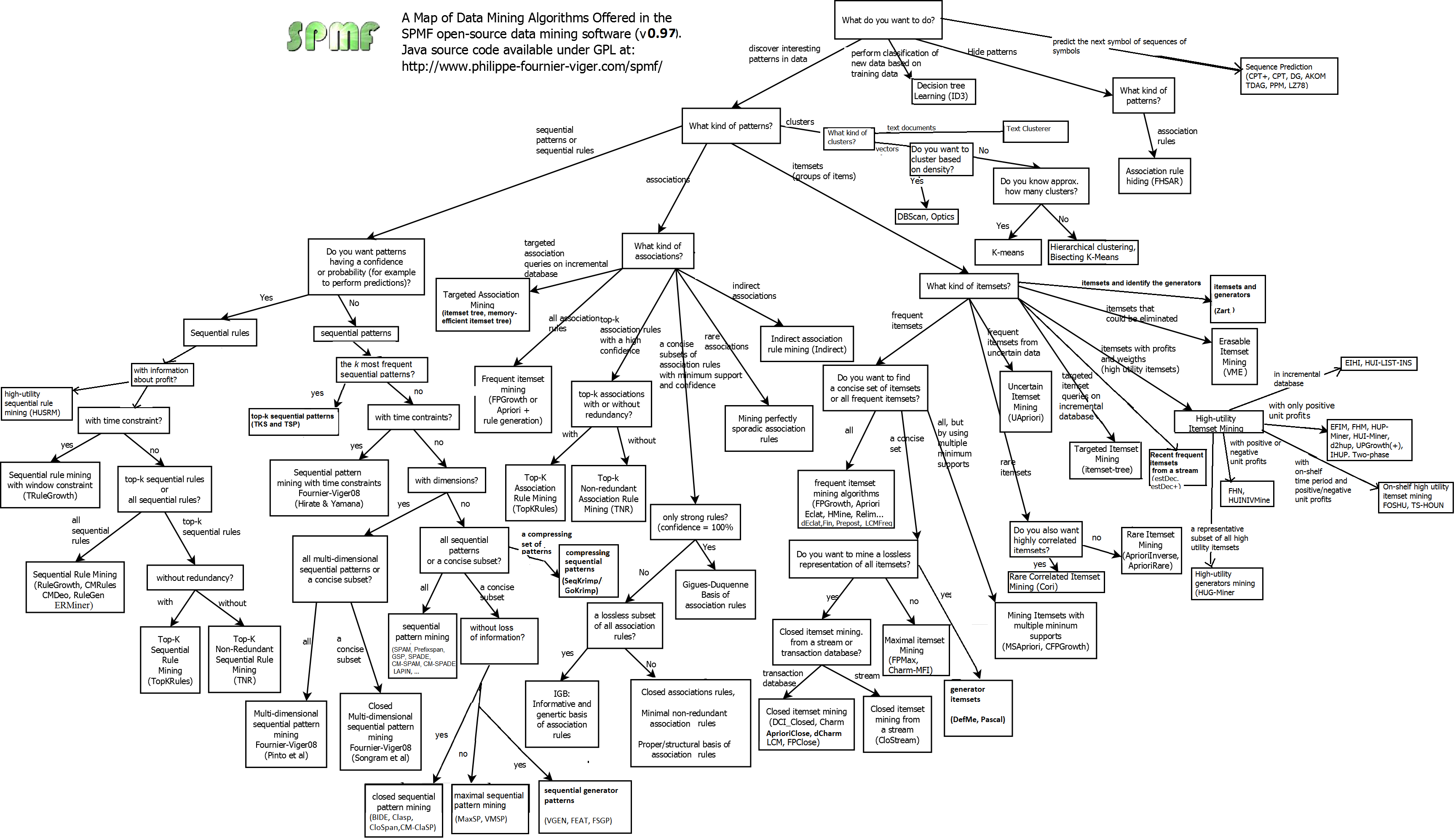
- [Java] SPMF, it contains many algorithms that cannot be found in R/Scikit-Learn/Spark, especailly algorithms about Pattern Mining: http://www.philippe-fournier-viger.com/spmf/index.php?link=algorithms.php
- [Python] Scikit-Learn algorithms map and Estimators
- map: http://scikit-learn.org/stable/tutorial/machine_learning_map/
- I'm sure that I have copied this before, but today I have learned something new about this map! Those green squares are clickable, and they are the estimators
- An estimator is used to help tune parameters and estimate the model
- This map also helps you find some algorithms in Scikit-Learn based on data size, data type
- [Python] TPOT - Automated Model Selection with Param Optimization
- TPOT documentation: http://rhiever.github.io/tpot/
- TPOT Python API: http://rhiever.github.io/tpot/api/
- It automatically does feature preprocessing, feature construction, feature selection, model selection and optimization
- For optimization, it is using Genetic Algorithm
- TPOT is built upon Scikit-Learn, so those models, methods you can find in TPOT can be found in scikit-learn too. This is what I really like. For example, in Scikit-Learn, classification will use stratfied cross validation while regression will use k-fold. TPOT does the same, and it helps you find the best model with optimized params in its pipeline
- [Python] MLBox - Automated Model Selection with Param Optimization
- MLBox GitHub: https://github.com/AxeldeRomblay/MLBox
- It does some data cleanning and preprocessing for you, but better to do things on your own before using it
- It also does model selction and param optimization like TPOT, what makes MLBox looks good is, each step of work, it ourputs some info to give you more insights of its performance
- MLBox Data Cleaning, in
train_test_split()- Delete unnamed cols
- Remove duplicates
- Extract month, year and day of the week from a Date column
- Remove Shifting Data automatically,
Drift_thresholder().fit_transform(data)- But it may be differ from manually removing shifting data, check my code here: https://github.com/hanhanwu/Hanhan_Data_Science_Practice/blob/master/deal_with_data_shifting.ipynb
- Only deals with covariate shifting (shifting in fetures)
- Details for how data shifting checking in MLBox works: https://www.analyticsvidhya.com/blog/2017/07/mlbox-library-automated-machine-learning/?utm_source=feedburner&utm_medium=email&utm_campaign=Feed%3A+AnalyticsVidhya+%28Analytics+Vidhya%29
- It uses Entity Embeding to enclode categorical data
- It seems that, with
Entity Encoding, you can link similar/relavant categorical values together
- It seems that, with
- Model Selection and Param Optimization
- It uses hyperopt library which is fast, below are the param categories you can set:
- Check params can be set in
optimize(): http://mlbox.readthedocs.io/en/latest/features.html#optimisation - Also check my code sample: https://github.com/hanhanwu/Hanhan_Data_Science_Practice/blob/master/try_mlbox.ipynb
- Shortages:
- Still in development, also some libraries used now can be out of dated in the next version
- No support to unsupervised learning for now
- [Python]Deploy Machine Learning Model as an API, using Flask: https://www.analyticsvidhya.com/blog/2017/09/machine-learning-models-as-apis-using-flask/?utm_source=feedburner&utm_medium=email&utm_campaign=Feed%3A+AnalyticsVidhya+%28Analytics+Vidhya%29
Statistics in Data Science
-
6 distributions
- Overall
- The expected value of any distribution is the mean of the distribution
- Bernoulli Distribution
- only 2 possible outcomes
- The expected value for a random variable X in this distributioon is
p(probability) - The variance for a random variable X in this distributioon is
p(1-p)
- Uniform Distributionz
- The probability of all the N number of outcomes are equally likely
a is min of uniform distribution,b is max of uniform distribution, the probability of a random variable in X is1/(b-a); the probability of a range (x1,x2) is(x2-x1)/(b-a)mean = (a+b)/2variance = (b-a)^2/12- Standard Uniform Distribution has
a=0, b=1, if x in [0,1] range, probability is 1, otherwise 0
- Binomial Distribution
- The probabilities for 2 outcomes are the same in each trail
- Each trail is independent
nis the number of trails,pis the probability of success in each trail =>mean=n*p,variance=n*p*(1-p)- If the probability of 2 outcomes are the same, then the distribution is normal distribution
- Normal Distribution
- The mean, median and mode of the distribution coincide.
- The curve of the distribution is bell-shaped and symmetrical about the line x=μ.
- The total area under the curve is 1.
- Exactly half of the values are to the left of the center and the other half to the right.
- Standard normal distribution has mean 0 and standard deviation 1
- Poisson Distribution
- It is applicable in situations where events occur at random points of time and space where in our interest lies only in the number of occurrences of the event.
- e.g number of times of have ice-cream in a year; number of flowers in a garden. etc
- Any successful event should not influence the outcome of another successful event.
- The probability of success over a short interval must equal the probability of success over a longer interval.
- The probability of success in an interval approaches zero as the interval becomes smaller.
λis the rate at which an event occurs,tis the length of a time interval, andXis the number of events in that time interval.mean = λ*t
- It is applicable in situations where events occur at random points of time and space where in our interest lies only in the number of occurrences of the event.
- Exponential Distribution
- Compared with poisson distribution, exponential distribution means the time interval between 2 events
- e.g the time interval between eating 2 ice-creams
- It is widely used in survival analysis.
λis called the failure rate of a device at any timet, given that it has survived up to t. For a random variable X,mean=1/λ,variance=(1/λ)^2. The greater the rate, the faster the curve drops and the lower the rate, flatter the curve.
- Compared with poisson distribution, exponential distribution means the time interval between 2 events
- Relationship between distributions
- Bernoulli Distribution is a special case of Binomial Distribution with a single trial
- Poisson Distribution is a limiting case of binomial distribution under the following conditions:
- The number of trials is indefinitely large or n → ∞.
- The probability of success for each trial is same and indefinitely small or p →0.
- np = λ, is finite
- Normal distribution is another limiting form of binomial distribution under the following conditions:
- The number of trials is indefinitely large, n → ∞
- Both p and q are NOT indefinitely small, and p=q
- Normal distribution is also a limiting case of Poisson distribution with the parameter λ →∞
- If the times between random events follow exponential distribution with rate λ, then the total number of events in a time period of length t follows the Poisson distribution with parameter λt.
- reference: https://www.analyticsvidhya.com/blog/2017/09/6-probability-distributions-data-science/?utm_source=feedburner&utm_medium=email&utm_campaign=Feed%3A+AnalyticsVidhya+%28Analytics+Vidhya%29
- Overall
-
Odds: Odds are defined as the ratio of the probability of success and the probability of failure. For example, a fair coin has probability of success is 1/2 and the probability of failure is 1/2 so odd would be 1
-
Bayesian Statistics
- Reference: https://www.analyticsvidhya.com/blog/2016/06/bayesian-statistics-beginners-simple-english/
- Frequentist Statistics
- Frequentist Statistics tests whether an event (hypothesis) occurs or not. It calculates the probability of an event in the long run of the experiment (i.e the experiment is repeated under the same conditions to obtain the outcome).
- Drawback 1 - p-value changes when sample size and stop intention change
- Drawback 2 - confidence level (C.L) also heavily depends on sample size like p-value
- Drawback 3 - confidence level (C.L) are not probability distributions therefore they do not provide the most probable value for a parameter and the most probable values
- Because of the drawbacks of Frequentist Statistics, here comes Bayesian Statistics
- "Bayesian statistics is a mathematical procedure that applies probabilities to statistical problems. It provides people the tools to update their beliefs in the evidence of new data."
- Bayes theorem is built on top of conditional probability and lies in the heart of Bayesian Inference.
- Bayes Theorem Wiki is better: https://en.wikipedia.org/wiki/Bayes%27_theorem
- Bayes Inference part here is good, especially in explaining
prior, likelyhood of observing prior, evidence and posterior. The probability of observing prior depends upon the fairness - The reason that we chose prior belief is to obtain a beta distribution. This is because when we multiply it with a likelihood function, posterior distribution yields a form similar to the prior distribution which is much easier to relate to and understand
- Bayes factor is the equivalent of p-value in the bayesian framework. The null hypothesis in bayesian framework assumes ∞ probability distribution only at a particular value of a parameter (say θ=0.5) and a zero probability else where. (M1); The alternative hypothesis is that all values of θ are possible, hence a flat curve representing the distribution. (M2).
Bayes factor is defined as the ratio of the posterior odds to the prior odds.To reject a null hypothesis, a BF <1/10 is preferred.
-
Find All Calculators here, this one is easier to understand and better to use
-
Termology glossary for statistics in machine learning: https://www.analyticsvidhya.com/glossary-of-common-statistics-and-machine-learning-terms/
-
Statistics behind Boruta feature selection: https://github.com/hanhanwu/Hanhan_Data_Science_Resources2/blob/master/boruta_statistics.pdf
-
How the laws of group theory provide a useful codification of the practical lessons of building efficient distributed and real-time aggregation systems (from 22:00, he started to talk about HyperLogLog and other approximation data structures): https://www.infoq.com/presentations/abstract-algebra-analytics
-
Confusing Concepts
- Errors and Residuals: https://en.wikipedia.org/wiki/Errors_and_residuals
- Heteroskedasticity: led by non-constant variance in error terms. Usually, non-constant variance is caused by outliers or extreme values
- Coefficient and p-value/t-statistics: coefficient measures the strength of the relationship of 2 variables, while p-value/t-statistics measures how strong the evidence that there is non-zero association
- Anscombe's quartet comprises four datasets that have nearly identical simple statistical properties, yet appear very different when graphed: https://en.wikipedia.org/wiki/Anscombe's_quartet
- Difference between gradient descent and stochastic gradient descent: https://www.quora.com/Whats-the-difference-between-gradient-descent-and-stochastic-gradient-descent
- Correlation & Covariance: In probability theory and statistics, correlation and covariance are two similar measures for assessing how much two attributes change together. The mean values of A and B, respectively, are also known as the expected values on A and B, E(A), E(B). Covariance, Cov(A,B)=E(A·B) - E(A)*E(B)
- Rate vs Proportion: A rate differs from a proportion in that the numerator and the denominator need not be of the same kind and that the numerator may exceed the denominator. For example, the rate of pressure ulcers may be expressed as the number of pressure ulcers per 1000 patient days.
-
Bias is useful to quantify how much on an average are the predicted values different from the actual value. A high bias error means we have a under-performing model which keeps on missing important trends. Varianc on the other side quantifies how are the prediction made on same observation different from each other. A high variance model will over-fit on your training population and perform badly on any observation beyond training.
-
OLS and Maximum likelihood are the methods used by the respective regression methods to approximate the unknown parameter (coefficient) value. OLS is to linear regression. Maximum likelihood is to logistic regression. Ordinary least square(OLS) is a method used in linear regression which approximates the parameters resulting in minimum distance between actual and predicted values. Maximum Likelihood helps in choosing the the values of parameters which maximizes the likelihood that the parameters are most likely to produce observed data.
-
Standard Deviation – It is the amount of variation in the population data. It is given by σ. Standard Error – It is the amount of variation in the sample data. It is related to Standard Deviation as σ/√n, where, n is the sample size, σ is the standandard deviation of the population. A low standard deviation indicates that the data points tend to be close to the mean (also called the expected value) of the set, while a high standard deviation indicates that the data points are spread out over a wider range of values. The standard deviation is the square root of the variance.
-
95% confidence interval does not mean the probability of a population mean to lie in an interval is 95%. Instead, 95% C.I means that 95% of the Interval estimates will contain the population statistic.
-
If a sample mean lies in the margin of error range then, it might be possible that its actual value is equal to the population mean and the difference is occurring by chance.
-
Difference between z-scores and t-values are that t-values are dependent on Degree of Freedom of a sample, and t-values use sample standard deviation while z-scores use population standard deviation.
-
The Degree of Freedom – It is the number of variables that have the choice of having more than one arbitrary value. For example, in a sample of size 10 with mean 10, 9 values can be arbitrary but the 10th value is forced by the sample mean.
-
Residual Sum of Squares (RSS) - It can be interpreted as the amount by which the predicted values deviated from the actual values. Large deviation would indicate that the model failed at predicting the correct values for the dependent variable. Regression (Explained) Sum of Squares (ESS) – It can be interpreted as the amount by which the predicted values deviated from the the mean of actual values.
-
Residuals is also known as the prediction error, they are vertical distance of points from the regression line
-
Co-efficient of Determination = ESS/(ESS + RSS). It represents the strength of correlation between two variables. Correlation Coefficient = sqrt(Co-efficient of Determination), also represents the strength of correlation between two variables, ranges between [-1,1]. 0 means no correlation, 1 means strong positive correlation, -1 means strong neagtive correlation.
-
About Data Sampling: http://psc.dss.ucdavis.edu/sommerb/sommerdemo/sampling/types.htm
- Probability sampling can be representative, non-probability sampling may not
- probability Sampling
* Random sample. (I guess R
sample()is random sampling by default, so that each feature has the same weight)- Stratified sample
- Nonprobability Sampling
- Quota sample
- Purposive sample
- Convenience sample
-
Comprehensive and Practical Statistics Guide for Data Science - A real good one!
- Sample Distribution and Population Distribution, Central Limit Theorem, Confidence Interval
- Hypothesis Testing
- t-test calculator
- ANOVA (Analysis of Variance), continuous and categorical variables, ANOVA also requires data from approximately normally distributed populations with equal variances between factor levels.
- F-ratio calculator
- Chi-square test, categorical variables
- chi-square calculator
- Regression and ANOVA, it is important is knowing the degree to which your model is successful in explaining the trend (variance) in dependent variable. ANOVA helps finding the effectiveness of regression models.
- An example of hypothesis test with chi-square:
- chi-square tests the hypothesis that A and B are independent, that is, there is no correlation between them. Chi-square is used to calculate the correlation between characteristical variables
- In this example, you have already calculated chi-square value as 507.93
- B feature has 2 levels, "science-fiction", "history"; A feature has 2 levels, "female", "male". So we can form a 2x2 table. The degree of freedom = (2-1)*(2-1) = 1
- Use the calculator here to calculate significant level, type degree of freedom as 1, probability as 0.001 (you can choose a probability you'd like). The calculated significant level is 10.82756617
- chi-square value 507.93 is much larger than the significant level, so we reject the hypothesis that A, B are independent and not correlated
-
Probability cheat sheet: http://www.cs.elte.hu/~mesti/valszam/kepletek
-
Likelihood vs Probability: http://mathworld.wolfram.com/Likelihood.html
- Likelihood is the hypothetical probability that a past event would yield a specific outcome.
- Probability refers to the occurrence of future events, while Likelihood refers to past events with known outcomes.
-
Probability basics with examples
- binonial distribution: a binomial distribution is the discrete probability distribution of the number of success in a sequence of n independent Bernoulli trials (having only yes/no or true/false outcomes).
- The normal distribution is perfectly symmetrical about the mean. The probabilities move similarly in both directions around the mean. The total area under the curve is 1, since summing up all the possible probabilities would give 1.
- Area Under the Normal Distribution
- Z score: The distance in terms of number of standard deviations, the observed value is away from the mean, is the standard score or the Z score. Observed value = µ+zσ [µ is the mean and σ is the standard deviation]
- Find Z Table here
-
Very Basic Conditional Probability and Bayes Theorem
- Independent, Exclusive, Exhaustive events
- Each time, when it's something about statistics pr probability, I will still read all the content to guarantee that I won't miss anything useful. This one is basic but I like the way it starts from simple concepts, using real life examples and finally leads to how does Bayes Theorem work. Although, there is an error in formula
P (no cancer and +) = P (no cancer) * P(+) = 0.99852*0.99, it should be0.99852*0.01 - There are some major formulas here are important to Bayes Theorem:
*
P(A|B) = P(A AND B)/P(B)P(A|B) = P(B|A)*P(A)/P(B)P(A AND B) = P(B|A)*P(A) = P(A|B)*P(B)P(b1|A) + P(b2|A) + .... + P(bn|A) = P(A)
-
Dispersion - In statistics, dispersion (also called variability, scatter, or spread) is the extent to which a distribution is stretched or squeezed. Common examples of measures of statistical dispersion are the variance, standard deviation, and interquartile range.
-
Common Formulas
- Examples: https://www.analyticsvidhya.com/blog/2017/05/41-questions-on-statisitics-data-scientists-analysts/?utm_source=feedburner&utm_medium=email&utm_campaign=Feed%3A+AnalyticsVidhya+%28Analytics+Vidhya%29
- About z-score
- When looking for probability, calculate z score first and check the value in the Z table, that value is the probability
- Observed value = µ+zσ [µ is the mean and σ is the standard deviation]
- Standard Error = σ/√N, [N is the number of Sample]; z = (Sample Mean - Population Mean)/Standard Error
- Find Z Table, t-distribution, chi-distribution here
- About t-score
- When compare 2 groups, calculate t-score
- t-statistic = (group1 Mean - group2 Mean)/Standard Error
- degree of freedom (df), if there are n sample, df=n-1 * t table with df, 1-tail, 2-tails and confidence level, compare your t-statistic with the relative value in this table, and decide whether to reject null hypothesis
- percentage of variability = t-statistic^2/(t-statistic^2 + degree of freedom) = correlation_coefficient ^2, so coefficient of determination equals to "percentage of variability"
- About F-statistic
- F-statistic is the value we receive when we run an ANOVA test on different groups to understand the differences between them.
- F-statistic = (sum of squared error for between group/degree of freedom for between group)/(sum of squared error for within group/degree of freedom for within group), as you can see from this formula, it cannot be negative
- Correlation
- Methods to calculate correlations between different data types: https://www.analyticsvidhya.com/blog/2016/01/guide-data-exploration/
- Formula to calculate correlation between 2 numerical variables (Question 28): https://www.analyticsvidhya.com/blog/2017/05/41-questions-on-statisitics-data-scientists-analysts/?utm_source=feedburner&utm_medium=email&utm_campaign=Feed%3A+AnalyticsVidhya+%28Analytics+Vidhya%29
- Correlation between the features won’t change if you add or subtract a constant value in the features.
- Significance level = 1- Confidence level
- Mean Absolute Error = the mean of absolute errors
- Normalization Methods
- min-max normalization = (x - min)/(max - min)
- z-score normalization = (x - mean)/standard deviation
- decimal scaling = x/1000, x/100, etc (depends on how could you make the values into [0,1] range)
-
Linear regression line attempts to minimize the squared distance between the points and the regression line. By definition the ordinary least squares (OLS) regression tries to have the minimum sum of squared errors. This means that the sum of squared residuals should be minimized. This may or may not be achieved by passing through the maximum points in the data. The most common case of not passing through all points and reducing the error is when the data has a lot of outliers or is not very strongly linear.
-
Person vs Spearman: Pearson correlation evaluated the linear relationship between two continuous variables. A relationship is linear when a change in one variable is associated with a proportional change in the other variable. Spearman evaluates a monotonic relationship. A monotonic relationship is one where the variables change together but not necessarily at a constant rate.
-
Coefficient
- Does similar work as correlation
- Tutorial to use it in Linear Regression: https://www.analyticsvidhya.com/blog/2017/06/a-comprehensive-guide-for-linear-ridge-and-lasso-regression/?utm_source=feedburner&utm_medium=email&utm_campaign=Feed%3A+AnalyticsVidhya+%28Analytics+Vidhya%29
-
Linear Algebra with Python calculations
- reference: https://www.analyticsvidhya.com/blog/2017/05/comprehensive-guide-to-linear-algebra/?utm_source=feedburner&utm_medium=email&utm_campaign=Feed%3A+AnalyticsVidhya+%28Analytics+Vidhya%29
- It talkes about those planes in linear algebra, matrix calculation
- What I like most is Eigenvalues and Eigenvectors part, because it's talking about how they related to machine learning. So Eigenvalues and Eigenvectors can be used in dimensional reduction such as PCA and reduce info loss.
- Singular Value Decomposition (SVD), used in removig redundant features, can be considered as a type of dimensional reduction too, but doesn't change the rest data as PCA does
-
To comapre the similarity between 2 curves
- Try to compare from these perspectives:
- Distance
- Shape
- Size of the Area in between
- Kolmogorov–Smirnov test - distance based
- its null hypothesis this, the smaple is drawn from the reference graph
- So, if the generated p-value is smaller than the threshold, reject null hypothesis, which means the 2 curves are not similar
- Dynamic Time Wrapping (DTW) - distance based
- Check the consistency of Peak and non-peak points of the 2 curves - shape based
- Try to compare from these perspectives:
-
Simulation Methods
- Monte Carlo Simulation: http://www.palisade.com/risk/monte_carlo_simulation.asp
- It can simulate all types of possible outcomes and probability of each outcome
- Monte Carlo Simulation: http://www.palisade.com/risk/monte_carlo_simulation.asp
-
Saddle Points
- The saddle point will always occur at a relative minimum along one axial direction (between peaks) and at a relative maximum along the crossing axis. Saddle Point Wiki
- How to Escape Saddle Point Efficiently
- Strict saddle points vs Non-strict saddle points: non-strict saddle points can be flat in the valley, strict saddle points require that there is at least one direction along which the curvature is strictly negative
- GD with only random initialization can be significantly slowed by saddle points, taking exponential time to escape. The behavior of PGD (projected GD) is strikingingly different — it can generically escape saddle points in polynomial time.
- Difference between Projected Gradient Descent (PGD) and Gradient Descent (GD)
Machine Learning Algorithms
-
KNN with R example: https://www.analyticsvidhya.com/blog/2015/08/learning-concept-knn-algorithms-programming/
- KNN unbiased and no prior assumption, fast
- It needs good data preprocessing such as missing data imputing, categorical to numerical
- k normally choose the square root of total data observations
- It is also known as lazy learner because it involves minimal training of model. Hence, it doesn’t use training data to make generalization on unseen data set.
-
SVM with Python example: https://www.analyticsvidhya.com/blog/2015/10/understaing-support-vector-machine-example-code/?utm_content=buffer02b8d&utm_medium=social&utm_source=facebook.com&utm_campaign=buffer
-
Basic Essentials of Some Popular Machine Learning Algorithms with R & Python Examples: https://www.analyticsvidhya.com/blog/2015/08/common-machine-learning-algorithms/?utm_content=buffer00918&utm_medium=social&utm_source=facebook.com&utm_campaign=buffer
- Linear Regression: Y = aX + b, a is slope, b is intercept. The intercept term shows model prediction without any independent variable. When there is only 1 independent variable, it is Simple Linear Regression, when there are multiple independent variables, it is Multiple Linear Regression. For Multiple Linear Regression, we can fit Polynomial Courvilinear Regression.
- When to use Ridge or Lasso: In presence of few variables with medium / large sized effect, use lasso regression. In presence of many variables with small / medium sized effect, use ridge regression. Lasso regression does both variable selection and parameter shrinkage, whereas Ridge regression only does parameter shrinkage and end up including all the coefficients in the model. In presence of correlated variables, ridge regression might be the preferred choice. Also, ridge regression works best in situations where the least square estimates have higher variance.
- Logistic Regression: it is classification, predicting the probability of discrete values. It chooses parameters that maximize the likelihood of observing the sample values rather than that minimize the sum of squared errors (like in ordinary regression).
- Decision Tree: serves for both categorical and numerical data. Split with the most significant variable each time to make as distinct groups as possible, using various techniques like Gini, Information Gain = (1- entropy), Chi-square. A decision tree algorithm is known to work best to detect non – linear interactions. The reason why decision tree failed to provide robust predictions because it couldn’t map the linear relationship as good as a regression model did.
- SVM: seperate groups with a line and maximize the margin distance. Good for small dataset, especially those with large number of features
- Naive Bayes: the assumption of equally importance and the independence between predictors. Very simple and good for large dataset, also majorly used in text classification and multi-class classification. Likelihood is the probability of classifying a given observation as 1 in presence of some other variable. For example: The probability that the word ‘FREE’ is used in previous spam message is likelihood. Marginal likelihood is, the probability that the word ‘FREE’ is used in any message.
- KNN: can be used for both classification and regression. Computationally expensive since it stores all the cases. Variables should be normalized else higher range variables can bias it. Data preprocessing before using KNN, such as dealing with outliers, missing data, noise
- K-Means
- Random Forest: bagging, which means if the number of cases in the training set is N, then sample of N cases is taken at random but with replacement. This sample will be the training set for growing the tree. If there are M input variables, a number m<<M is specified such that at each node, m variables are selected at random out of the M and the best split on these m is used to split the node. The value of m is held constant during the forest growing. Each tree is grown to the largest extent possible. There is no pruning. Random Forest has to go with cross validation, otherwise overfitting could happen.
- PCA: Dimensional Reduction, it selects fewer components (than features) which can explain the maximum variance in the data set, using Rotation. Personally, I like Boruta Feature Selection. Filter Methods for feature selection are my second choice. Remove highly correlated variables before using PCA
- GBM (try C50, XgBoost at the same time in practice)
- Difference between Random Forest and GBM: Random Forest is bagging while GBM is boosting. In bagging technique, a data set is divided into n samples using randomized sampling. Then, using a single learning algorithm a model is build on all samples. Later, the resultant predictions are combined using voting or averaging. Bagging is done is parallel. In boosting, after the first round of predictions, the algorithm weighs misclassified predictions higher, such that they can be corrected in the succeeding round. This sequential process of giving higher weights to misclassified predictions continue until a stopping criterion is reached.Random forest improves model accuracy by reducing variance (mainly). The trees grown are uncorrelated to maximize the decrease in variance. On the other hand, GBM improves accuracy my reducing both bias and variance in a model.
-
Online Learning vs Batch Learning: https://www.analyticsvidhya.com/blog/2015/01/introduction-online-machine-learning-simplified-2/
-
Optimization - Genetic Algorithm
- More about Crossover and Mutation: https://www.researchgate.net/post/What_is_the_role_of_mutation_and_crossover_probability_in_Genetic_algorithms
-
Survey of Optimization
- Page 10, strength and weakness of each optimization method: https://github.com/hanhanwu/readings/blob/master/SurveyOfOptimization.pdf
-
Optimization - Gradient Descent
- Reference: https://www.analyticsvidhya.com/blog/2017/03/introduction-to-gradient-descent-algorithm-along-its-variants/?utm_source=feedburner&utm_medium=email&utm_campaign=Feed%3A+AnalyticsVidhya+%28Analytics+Vidhya%29
- Challenges for gradient descent
- data challenge: cannot be used on non-convex optimization problem; may end up at local optimum instead of global optimum; may even not an optimal point when gradient is 0 (saddle point)
- gradient challenge: when gradient is too small or too large, vanishing gradient or exploding gradient could happen
- implementation chanllenge: memory, hardware/software limitations
- Type 1 - Vanilla Gradient Descent
- "Vanilla" means pure here
update = learning_rate * gradient_of_parametersparameters = parameters - update
- Type 2 - Gradient Descent with Momentum
update = learning_rate * gradientvelocity = previous_update * momentumparameter = parameter + velocity – update- With
velocity, it considers the previous update
- Type 3 - ADAGRAD
- ADAGRAD uses adaptive technique for learning rate updation.
grad_component = previous_grad_component + (gradient * gradient)rate_change = square_root(grad_component) + epsilonadapted_learning_rate = learning_rate * rate_changeupdate = adapted_learning_rate * gradientparameter = parameter – updateepsilonis a constant which is used to keep rate of change of learning rate
- Type 4 - ADAM
- ADAM is one more adaptive technique which builds on adagrad and further reduces it downside. In other words, you can consider this as momentum + ADAGRAD.
adapted_gradient = previous_gradient + ((gradient – previous_gradient) * (1 – beta1))gradient_component = (gradient_change – previous_learning_rate)adapted_learning_rate = previous_learning_rate + (gradient_component * (1 – beta2))update = adapted_learning_rate * adapted_gradientparameter = parameter – update
- Tips for choose models
- For rapid prototyping, use adaptive techniques like Adam/Adagrad. These help in getting quicker results with much less efforts. As here, you don’t require much hyper-parameter tuning.
- To get the best results, you should use vanilla gradient descent or momentum. gradient descent is slow to get the desired results, but these results are mostly better than adaptive techniques.
- If your data is small and can be fit in a single iteration, you can use 2nd order techniques like l-BFGS. This is because 2nd order techniques are extremely fast and accurate, but are only feasible when data is small enough
Data Visualization
-
Previous Visualization collections, check "VISUALIZATION" section: https://github.com/hanhanwu/Hanhan_Data_Science_Resources/blob/master/README.md
-
Readings
- Psychology of Intelligence Analysis: https://www.cia.gov/library/center-for-the-study-of-intelligence/csi-publications/books-and-monographs/psychology-of-intelligence-analysis/PsychofIntelNew.pdf
- How to lie with Statistics: http://www.horace.org/blog/wp-content/uploads/2012/05/How-to-Lie-With-Statistics-1954-Huff.pdf
- The Signal and the Noise (to respect the author): https://www.amazon.com/Signal-Noise-Many-Predictions-Fail-but/dp/0143125087/ref=sr_1_1?ie=UTF8&qid=1488403387&sr=8-1&keywords=signal+and+the+noise
- Non-designer's design book: https://diegopiovesan.files.wordpress.com/2010/07/livro_-_the_non-designers_desi.pdf
-
Python LIME - make machine learning models more readable
- This was why I chose HCI in my last semester. Many people are working on visualization methods to make machine learning models more interpretable. This is good, especially when you are working in the industry, business leaders, customers or even techinical people all prefer an easy-to-understand way.
- This python library focuses on interpreting classification models now. Majorly about indicating which features contribute to which class
- Open source: https://github.com/marcotcr/lime
- Code examples: https://www.analyticsvidhya.com/blog/2017/06/building-trust-in-machine-learning-models/?utm_source=feedburner&utm_medium=email&utm_campaign=Feed%3A+AnalyticsVidhya+%28Analytics+Vidhya%29
- I didn't try the code because it does not contain clustering. And in fact confusion matrix is easier for me to understand, compared with their visualization, and it cannot tell the feature rankings for their contributions to the prediction. But their ideas are still a good start, they have converted decision tree ideas into other classification interpretation.
-
NLP Visualization
- On Jan 20, 2017, SFU Linguistics Lab invited an UBC researcher to show NLP data visualization, which is very interesting. By doing topic modeling, graph base clustering, they are able to categorize large amount of comments and opinions into groups, by using interactive visualization, the tools they developed will help readers read online comments in a more efficient way.
- ConVis: https://www.cs.ubc.ca/cs-research/lci/research-groups/natural-language-processing/ConVis.html
- MultiConVis: https://www.cs.ubc.ca/cs-research/lci/research-groups/natural-language-processing/MultiConVis.html
-
Python Bokeh, an open source data visualization tool (its presentation target is web browser, but I think Tableau and d3 all could do this): https://www.analyticsvidhya.com/blog/2015/08/interactive-data-visualization-library-python-bokeh/?utm_content=buffer58668&utm_medium=social&utm_source=plus.google.com&utm_campaign=buffer
-
Tableau Resources
- Reference Guide: http://www.dataplusscience.com/TableauReferenceGuide/
- Advanced Highlight: http://onlinehelp.tableau.com/current/pro/desktop/en-us/actions_highlight_advanced.html
- Having 1+ pills in Color: http://drawingwithnumbers.artisart.org/measure-names-on-the-color-shel/
- Mark Labels: http://onlinehelp.tableau.com/current/pro/desktop/en-us/annotations_marklabels_showhideindividual.html
- Show or hide labels: http://paintbynumbersblog.blogspot.ca/2013/08/a-quick-tableau-tip-showing-and-hiding.html
- Filter and parameter: https://www.quora.com/What-is-the-difference-between-filters-and-parameters-in-a-tableau-What-is-an-explanation-of-this-scenario
- Tableau detailed user guide on parameter: http://onlinehelp.tableau.com/current/pro/desktop/en-us/help.html#parameters_swap.html
- Logincal function: http://onlinehelp.tableau.com/current/pro/desktop/en-us/functions_functions_logical.html
- Tableau functions: http://onlinehelp.tableau.com/current/pro/desktop/en-us/functions.html
-
Jigsaw - Data Visualization for text data
- Tutorial Videos (each video is very short, good): http://www.cc.gatech.edu/gvu/ii/jigsaw/tutorial/
- Jigsaw manual: http://www.cc.gatech.edu/gvu/ii/jigsaw/tutorial/manual/#initiating-session
-
Gephi
- It create interactive graph-network visualization
- Tutorials: https://gephi.org/users/
- This is a sample data input, showing what kind of data structure you need for visualizing network in Grphi, normally, 2 files, one for Nodes one for Edges: https://github.com/hanhanwu/Hanhan_Data_Science_Resources2/blob/master/gephi%20data%20set.zip
- With the dataset I give you here, you will be able to find girls dinning group at school and make assumptions about how rumor spreaded (network is so scary, right?)
- Here is what I listed about the advantages of using Gephi for network visualization, compared with writing python visualization: https://github.com/hanhanwu/Hanhan_Data_Science_Resources2/blob/master/gephi.png
- But something is wrong with the Gephi on my machine.. I don't have partition or ranking settings and cannot choose dirested graph and so on...
- However, seeing the changes of those vosualization with different graph algorithm is interesting, for example, Force Atlas 2: https://github.com/gephi/gephi/wiki/Force-Atlas-2
-
MicrosoStrategy - Visual Analytics Course List: https://www.microstrategy.com/us/services/education/course-list#filter-role:path=default|filter-platform:path=default|filter-version:path=._10_5|filter-certification:path=default|sort-course-number:path~type~order=.card-corner~text~asc
-
Python Elastic Search & Kibana for data visualization: https://www.analyticsvidhya.com/blog/2017/05/beginners-guide-to-data-exploration-using-elastic-search-and-kibana/?utm_source=feedburner&utm_medium=email&utm_campaign=Feed%3A+AnalyticsVidhya+%28Analytics+Vidhya%29
- I still prefer R or Spark for visualized data exploration, if you care about the speed. otherwise, tableau
- "Elastic Search is an open source, RESTful distributed and scalable search engine. Elastic search is extremely fast in fetching results for simple or complex queries on large amounts of data (Petabytes) because of it’s simple design and distributed nature. It is also much easier to work with than a conventional database constrained by schemas, tables."
- The tutorial prevides the method to indexing the data for Elastic Search
-
My d3 Practice
Big Data
- Pig vs Hive: https://upxacademy.com/pig-vs-hive/
- Spark 2.0, SparkSession (can be used for both Spark SQL Context and Hive Context, Spark SQL is based on Haive but has its own strength): http://cdn2.hubspot.net/hubfs/438089/notebooks/spark2.0/SparkSession.html
- Mastering Spark 2.0: https://github.com/hanhanwu/Hanhan_Data_Science_Resources2/blob/master/Mastering-Apache-Spark-2.0.pdf
- Spark Session - supports both SQL Context and Hive Context
- Structured Streaming - just write batch computation and let Spark deal with streaming with you. I’m waiting to see its better integration with MLLib and other machine learning libraries
- HyperLogLog - the story is interesting
val ds = spark.read.json("/databricks-public-datasets/data/iot/iot_devices.json").as[DeviceIoTData]- Choice of Spark DataFrame, DataSets and RDD, P35
- Structured Streaming, P57-59
- Lessons from large scale machine learning deployment on Spark, 2.0: https://github.com/hanhanwu/Hanhan_Data_Science_Resources2/blob/master/Lessons_from_Large-Scale_Machine_Learning_Deployments_on_Spark.pdf
- Hadoop 10 years: https://upxacademy.com/hadoop-10-years/
- Why Cloud Service is better than HDFS: https://databricks.com/blog/2017/05/31/top-5-reasons-for-choosing-s3-over-hdfs.html?utm_campaign=Company%20Blog&utm_content=55155959&utm_medium=social&utm_source=linkedin
- Hive function cheat sheet: https://www.qubole.com/resources/cheatsheet/hive-function-cheat-sheet/
- Distributing System
- Spack New Physical Plan: https://databricks.com/blog/2017/04/01/next-generation-physical-planning-in-apache-spark.html?utm_campaign=Databricks&utm_content=51844317&utm_medium=social&utm_source=linkedin
- CAP Theorem: https://en.wikipedia.org/wiki/CAP_theorem
- CAPP: https://drive.google.com/file/d/0B3Um1hpy8q7gVjhVT3dGUWFxRm8/view
- S survey summary on NoSQL: https://www.linkedin.com/pulse/survey-nosql-key-value-pair-databases-uzma-ali-pmp?trk=v-feed&lipi=urn%3Ali%3Apage%3Ad_flagship3_feed%3BspSXDtIY3PN6lbk4C%2FTwTg%3D%3D
- I like the summary table in this poster
- They did survey on Cassandra, Redis, DynamoDB, Riak, HBASE, Voldemort (among them, I have only used HBASE so far...)
- A book - I Heart Logs
- The book: https://github.com/hanhanwu/readings/blob/master/I_Heart_Logs.pdf
- It talks about how powerful logs can be in distributing systems, streaming processing, etc, each section has a real-life example. I like the streaming processing part in this book most.
- It is a great book that has broaden and deepen the concepts we have heard many time times but may has misunderstanding, such as "logs", "streaming processing" and even "ETL".
- Google Caffeine: https://googleblog.blogspot.ca/2010/06/our-new-search-index-caffeine.html
- It rebuilt its web crawling, processing, and indexing pipeline—what has to be one of the most complex, largest scale data processing systems on the planet —on top of a stream processing system.
- NoSQL
- CAP theorem (could only choose 2)
- Consistency: all clients always have the same view of data
- Avability: client can always read and write
- Partition tolerance means that the system works well across physical network partitions
- There are different types of NoSql databases
- Column oriented
- Documented oriented
- Graph database
- Key-value oriented
- NoSql visual guide: http://blog.nahurst.com/visual-guide-to-nosql-systems
- Some other description: http://stackoverflow.com/questions/2798251/whats-the-difference-been-nosql-and-a-column-oriented-database
- Amazon DynamoDB vs. Amazon Redshift vs. Oracle NoSQL: https://db-engines.com/en/system/Amazon+DynamoDB%3BAmazon+Redshift
- It seems that DynamoDB is NoSql while Redshift is a data warehouse based on psql
- CAP theorem (could only choose 2)
Cloud
-
For Cloud Machine Learning in Spark, AWS and Azure Machine Learning, check my previous summary here: https://github.com/hanhanwu/Hanhan_Data_Science_Resources
-
My AWS practice: https://github.com/hanhanwu/Hanhan_AWS
-
Compute Canada & West Grid
- How to apply for an account: https://www.computecanada.ca/research-portal/account-management/apply-for-an-account/
- login West Grid cloud through terminal: https://www.westgrid.ca//support/quickstart/new_users#about
- Note: the GUI the above guidance mentioned means the graphical tool, not interactive user interface...
- Run X11 in Mac OS X with XQuartz: http://osxdaily.com/2012/12/02/x11-mac-os-x-xquartz/
- When you are using XQuartz, once xterm appeared, loggin into Canada Computer with SSH X forwarding through xterm: https://www.westgrid.ca/support/visualization/remote_visualization/x11
- Creat Computer Canada Cloud (it seems that Computer Canada Cloud and West Grid are different cloud, but you apply for West Grid through Compute Canada account): https://www.computecanada.ca/research-portal/national-services/compute-canada-cloud/create-a-cloud-account/
- Tutorial for creating Compute Canada cloud (the video at the bottom): https://www.computecanada.ca/research-portal/national-services/compute-canada-cloud/
- Cloud Canada Quick Start: https://docs.computecanada.ca/wiki/Cloud_Quick_Start
- Command lines: https://github.com/hanhanwu/Hanhan_Data_Science_Resources2/blob/master/WestGrid_commands.md
TEXT ANALYSIS
- Text data preprocessing basic steps: https://www.analyticsvidhya.com/blog/2015/06/quick-guide-text-data-cleaning-python/
- My NLP practice: https://github.com/hanhanwu/Hanhan_NLP
- Jigsaw - Data Visualization for text data
- Tutorial Videos (each video is very short, good): http://www.cc.gatech.edu/gvu/ii/jigsaw/tutorial/
- Jigsaw manual: http://www.cc.gatech.edu/gvu/ii/jigsaw/tutorial/manual/#initiating-session
Non-Machine Learning Data Analysis Examples
- Analysis with data visualization: https://www.analyticsvidhya.com/blog/2016/12/who-is-the-superhero-of-cricket-battlefield-an-in-depth-analysis/?utm_source=feedburner&utm_medium=email&utm_campaign=Feed%3A+AnalyticsVidhya+%28Analytics+Vidhya%29
AI
-
BOOK - Fundamentals of Deep Learning: https://github.com/hanhanwu/readings/blob/master/fundamentals-of-deep-learning-sampler.pdf
- I found the full book in school library, it should be able to be found at Microsoft library too :)
-
Course - Standford Convolutional Network for Visual Recognition: http://cs231n.github.io/convolutional-networks/
- Younger kids are so lucky nowadays! I found the notes are pretty good to review important concepts that will be used in neural network implemention. Now let me review some courses here, otherwise it really gives me lots of difficulties in debugging CNN
- Demo architecture, 10 class classification: http://cs.stanford.edu/people/karpathy/convnetjs/demo/cifar10.html
- My notes: https://github.com/hanhanwu/Hanhan_Data_Science_Resources2/blob/master/Standford_CNN_Notes1.pdf
-
Neural Network is an Universal Approximators. Besides, Kernel SVM and Boosted Decision Trees are also universal approximators
-
Deep Learning basic concepts (it's a real good one!): https://www.analyticsvidhya.com/blog/2017/05/25-must-know-terms-concepts-for-beginners-in-deep-learning/?utm_source=feedburner&utm_medium=email&utm_campaign=Feed%3A+AnalyticsVidhya+%28Analytics+Vidhya%29
- how does
activation functionwork: *u = ∑W*X+b, X is the input vector, W is the weights vector, b is bias- apply activation function
f()to u,f(u)is the output of the layer
- apply activation function
- Different activation functions
- The sigmoid transformation generates a more smooth range of values between 0 and 1. We might need to observe the changes in the output with slight changes in the input values. Smooth curves allow us to do that and are hence preferred over step functions.
- The major benefit of using ReLU is that it has a constant derivative value for all inputs greater than 0. The constant derivative value helps the network to train faster.
- softmax, normally used in the output layer for classification. It is similar to sigmoid but its output is normalized to make the sum as 1. Meanwhile, sigmoid is used for binary classification while softmax can be used on multi-class classification.
- Gradient Descent & Optimization & Cost function: Gradient descent is an optimization method, aiming at minimizing the cost/loss
- Backpropagation is used to update weights
- Batches: While training a neural network, instead of sending the entire input in one go, we divide in input into several chunks of equal size randomly. Training the data on batches makes the model more generalized as compared to the model built when the entire data set is fed to the network in one go.
- Epochs: An epoch is defined as a single training iteration of all batches in both forward and back propagation. This means 1 epoch is a single forward and backward pass of the entire input data. Higher epochs could lead to higher accuracy but maybe also overfitting, the higher one also takes longer time.
- Dropout: Dropout is a regularization technique which prevents over-fitting of the network. When training a certain number of neurons in the hidden layer is randomly dropped. This means that the training happens on several architectures of the neural network on different combinations of the neurons. You can think of drop out as an ensemble technique, where the output of multiple networks is then used to produce the final output.
- Batch Normalization, it is used to ensure the data distribution will be the same as the next layer expected. Because after backpropagation, the weights changed and the data distribution may also changed while te next layer expects to see similar data distribution it has seen before.
- CNN (Convolutional Neural Network)
- 1×1 convolution CNN can help in dimensionality reduction, feature pooling and it suffers less overfitting due to small kernel size
- Filter: is a smaller window of data, it used to filter the entire data into multiples windows, each window generates a convoluted value. All the convoluted values form a new set of data. Using this method, an image can be convoluted into less parameters. CNN is often used on image
- Pooling: a pooling layer is often added between convolutional layers to reduce parameters in order to reduce overfitting. For example, in practice, MAX pooling works better
- Padding: Padding refers to adding extra layer of zeros across the images so that the output image has the same size as the input
- Data Augmentation: the addition of new data derived from the given data, which might prove to be beneficial for prediction. Such as brightening/rotating the image
- Detailed CNN Go Through: https://www.analyticsvidhya.com/blog/2017/06/architecture-of-convolutional-neural-networks-simplified-demystified/?utm_source=feedburner&utm_medium=email&utm_campaign=Feed%3A+AnalyticsVidhya+%28Analytics+Vidhya%29
- Not a big fan of deep learning, but I am paying attention to all these tuutorials as well, to learn more about them. This article is a real good one. I love this typy of go through, from the very beginning, step by step, telling you how an algorithm work, with examples :)
- CNN is a popular algorithm for image classification
- Images are formed by pixels, if the order or color of these pixels change, the image will change too. Machine will break an image into a matrix of pixels, and store the color code of each pixel at the representative position
- A fully connected network would take this image as an array by flattening it and considering pixel values as features to predict the number in image. What CNN does is to take the input image, define a weight matrix and the input is convolved to extract specific features from the image without losing the information about its spatial arrangement, this also significantly reduces number of features
- The convolution layer - kk matrix with 0,1 weights, use this kK matrix in the whole n*n matrix to extract features. Weights are learnt such that the loss function will be minimized. When there are multiple convolution layer, the deeper the layer is, the more complex features it extratced. An activation map is the output of the convolution layer.
- Stride: If the weight matrix moves 1 pixel at a time, we call it as a stride of 1. The size of image keeps on reducing as we increase the stride value
- Padding: Padding the input image with zeros across it when the size shrinked after stride. This is to preserve the size of the image
- The spatial size of the output image can be calculated as
([W-F+2P]/S)+1. Here, W is the input volume size, F is the size of the filter, P is the number of padding applied and S is the number of strides. - Output Layer - The convolution and pooling layers would only be able to extract features and reduce the number of parameters from the original images. However, to generate the final output we need to apply a fully connected layer to generate an output equal to the number of classes we need. The output layer has a loss functionlike categorical cross-entropy, to compute the error in prediction. Once the forward pass is complete the backpropagation begins to update the weight and biases for error and loss reduction.
- Images should be resized to the same shape and size before using CNN. You can use Python
cv2for image resizing.images[i]=cv2.resize(images[i],(300,300))
- RNN (Recurrent Neural Network)
- Recurrent Neuron: A recurrent neuron is one in which the output of the neuron is sent back to it for t time stamps.
- RNN is often used for sequential data, such as time series
- Vanishing Gradient Problem – Vanishing gradient problem arises in cases where the gradient of the activation function is very small. During back propagation when the weights are multiplied with these low gradients, they tend to become very small and “vanish” as they go further deep in the network. This makes the neural network to forget the long range dependency. This generally becomes a problem in cases of recurrent neural networks where long term dependencies are very important for the network to remember. This can be solved by using activation functions like ReLu which do not have small gradients.
- Exploding Gradient Problem – This is the exact opposite of the vanishing gradient problem, where the gradient of the activation function is too large. During back propagation, it makes the weight of a particular node very high with respect to the others rendering them insignificant. This can be easily solved by clipping the gradient so that it doesn’t exceed a certain value.
- how does
-
Computer Vision & Deep Learning Architectures
- https://www.analyticsvidhya.com/blog/2017/08/10-advanced-deep-learning-architectures-data-scientists/?utm_source=feedburner&utm_medium=email&utm_campaign=Feed%3A+AnalyticsVidhya+%28Analytics+Vidhya%29
- Computer Vision Tasks:
- Object Recognition / classification
- Classification + Localisation
- Object Detection
- Image Segmentation
- Architectures
- AlexNet: a simple architecture with convolutional and pooling layers one on top of the other, followed by fully connected layers at the top. AlexNet speeds up the training by 10 times just by the use of GPU.
- VGG Net: characterized by its pyramidal shape, where the bottom layers which are closer to the image are wide, whereas the top layers are deep. It contains subsequent convolutional layers followed by pooling layers. It is very slow to train if trained from scratch, even on a decent GPU. But pre-trained networks for VGG are available freely on the internet, so it is commonly used out of the box for various applications.
- GoogleNet: made a novel approach called the Inception Module. It is a drastic change from the sequential architectures. In a single layer, multiple types of “feature extractors” are present. The network at training itself has many options to choose from when solving the task. It can either choose to convolve the input, or to pool it directly. GoogleNet trains faster than VGG. Size of a pre-trained GoogleNet is comparatively smaller than VGG.
- ResNet: consists of multiple subsequent residual modules, which are the basic building block of ResNet architecture. A residual module has two options, either it can perform a set of functions on the input, or it can skip this step altogether. Similar to GoogleNet, these residual modules are stacked one over the other to form a complete end-to-end network. The main advantage of ResNet is that hundreds, even thousands of these residual layers can be used to create a network and then trained. This is a bit different from usual sequential networks, where you see that there is reduced performance upgrades as you increase the number of layers.
- ResNeXt: the improvement on ResNet. A current state-of-art technique in object recognition
- RCNN (Region Based CNN): It is said to be the most influential of all the deep learning architectures that have been applied to object detection problem. It attempts to draw a bounding box over all the objects present in the image, and then recognize what object is in the image with CNN.
- YOLO (You Only Look Once): First of all, I like this name. A current state-of-the-art real time system built on deep learning for solving image detection problems. It first divides the image into defined bounding boxes, and then runs a recognition algorithm in parallel for all of these boxes to identify which object class do they belong to. All of this is done in parallely, so it can run in real time; processing upto 40 images in a second.
- SqueezeNet: extremely useful in low bandwidth scenarios like mobile platforms. It using a specialized structure called the fire module.
- SegNet: it deals with image segmentation problem. It consists of sequence of processing layers (encoders) followed by a corresponding set of decoders for a pixelwise classification. The information transfer is direct instead of convolving them.
- GAN (Generative Adversarial Network): It is used to generate an entirely new image which is not present in the training dataset, but is realistic enough to be in the dataset.
- Reference (good one!): https://www.analyticsvidhya.com/blog/2017/08/10-advanced-deep-learning-architectures-data-scientists/?utm_source=feedburner&utm_medium=email&utm_campaign=Feed%3A+AnalyticsVidhya+%28Analytics+Vidhya%29
- An example to build atchitecture in Keras (Step 7): https://elitedatascience.com/keras-tutorial-deep-learning-in-python#step-7
-
NN examples in R and Python: https://www.analyticsvidhya.com/blog/2017/05/neural-network-from-scratch-in-python-and-r/?utm_source=feedburner&utm_medium=email&utm_campaign=Feed%3A+AnalyticsVidhya+%28Analytics+Vidhya%29
-
Use pre-trained model for deep learning: https://www.analyticsvidhya.com/blog/2017/06/transfer-learning-the-art-of-fine-tuning-a-pre-trained-model/?utm_source=feedburner&utm_medium=email&utm_campaign=Feed%3A+AnalyticsVidhya+%28Analytics+Vidhya%29
-
Deep Learning talks from PyData (it also has some other data science talks): https://www.analyticsvidhya.com/blog/2017/05/pydata-amsterdam-2017-machine-learning-deep-learning-data-science/?utm_source=feedburner&utm_medium=email&utm_campaign=Feed%3A+AnalyticsVidhya+%28Analytics+Vidhya%29
-
Neural Network vs Deep Learning: When there are more hidden layers and increase depth of neural network a neural network becomes deep learning.
-
Something about AI (those brief explaination about real life applications are useful and intresting): https://www.analyticsvidhya.com/blog/2016/12/artificial-intelligence-demystified/?utm_source=feedburner&utm_medium=email&utm_campaign=Feed%3A+AnalyticsVidhya+%28Analytics+Vidhya%29
-
Deep Learning Learning Resources: https://www.analyticsvidhya.com/blog/2016/08/deep-learning-path/
-
Reinforcement Learning Open Sources: https://www.analyticsvidhya.com/blog/2016/12/getting-ready-for-ai-based-gaming-agents-overview-of-open-source-reinforcement-learning-platforms/?utm_source=feedburner&utm_medium=email&utm_campaign=Feed%3A+AnalyticsVidhya+%28Analytics+Vidhya%29
-
Reinforcement Learning with Python Example: https://www.analyticsvidhya.com/blog/2017/01/introduction-to-reinforcement-learning-implementation/?utm_source=feedburner&utm_medium=email&utm_campaign=Feed%3A+AnalyticsVidhya+%28Analytics+Vidhya%29
-
Deeping Learning APIs, help you build simple apps (it's interesting): https://www.analyticsvidhya.com/blog/2017/02/6-deep-learning-applications-beginner-python/?utm_source=feedburner&utm_medium=email&utm_campaign=Feed%3A+AnalyticsVidhya+%28Analytics+Vidhya%29
-
5 More Deep Learning APIs [Python]: https://www.analyticsvidhya.com/blog/2017/02/5-deep-learning-applications-beginner-python/?utm_source=feedburner&utm_medium=email&utm_campaign=Feed%3A+AnalyticsVidhya+%28Analytics+Vidhya%29
-
Deep Learning Skillset Test1: https://www.analyticsvidhya.com/blog/2017/01/must-know-questions-deep-learning/?utm_source=feedburner&utm_medium=email&utm_campaign=Feed%3A+AnalyticsVidhya+%28Analytics+Vidhya%29
- Neural Networks cannot do data preprocessing themselves
- Neural Network Dropout can be seen as an extreme form of Bagging in which each model is trained on a single case and each parameter of the model is very strongly regularized by sharing it with the corresponding parameter in all the other models.
- Neural Network uses hidden layers to reduce dimensionality, it is based on predictive capability of the features. By comparison, PCA does dimensional reduction based on feature correlation
- People set a metric called bayes error which is the error they hope to achieve, this is because: Input variables may not contain complete information about the output variable; System (that creates input-output mapping) may be stochastic; Limited training data
- The number of neurons in the output layer dose NOT have to match the number of classes. If your outputis using one-hot encoding, they have to match. Otherwise, you can use other methods. For example, 2 neurons represent 4 classes using binary bits (00, 01, 10, 11)
- Without knowing what are the weights and biases of a neural network, we cannot comment on what output it would give.
- Convolutional Neural Network would be better suited for image related problems because of its inherent nature for taking into account changes in nearby locations of an image
- Recurrent neural network works best for sequential data. Recurrent neuron can be thought of as a neuron sequence of infinite length of time steps. Dropout does not work well with recurrent layer.
- A neural network is said to be a universal function approximator, so it can theoretically represent any decision boundary.
- To decrease the “ups and downs” when visualizing errors, you can try to increase the batch size. But the "ups and downs" are no need to worry as long as there is a cumulative decrease in both training and validation error.
- When you want to re-use a pre-trained NN model on similar problems, you can keep the previous layers but only re-train the last layer, since all the previous layers work as feature extractors
- To deal with overfitting in NN, you can use Dropout, Regularization and Batch Normalization. Using Batch Normalization is possbile to reach higher level accuracy. Dropout is designed as a regulazer in order to reduce the gap between the tester and the trainer; Batch Normalization is designed to make optimization easier, so it does less regularization. So Batch Normalization is not as strong as dropout. When the dataset is very small, Dropout should be better than Batch Normalization. Batch Normalization video: https://www.youtube.com/watch?v=Xogn6veSyxA
-
Deep Learning Skillset Test2: https://www.analyticsvidhya.com/blog/2017/04/40-questions-test-data-scientist-deep-learning/?utm_source=feedburner&utm_medium=email&utm_campaign=Feed%3A+AnalyticsVidhya+%28Analytics+Vidhya%29
- NN is a representative algorithm, which means: it converts data to a form that better solve the problem
- Perplexity is a commonly used evaluation technique when applying deep learning for NLP tasks. Lower the perplexity the better.
- Sigmoid was the most commonly used activation function in neural network, until an issue was identified. The issue is that when the gradients are too large in positive or negative direction, the resulting gradients coming out of the activation function get squashed. This is called saturation of the neuron. That is why ReLU function was proposed, which kept the gradients same as before in the positive direction. ReLU also gets saturated, but it's on the negative side of x-axis.
- Dropout Rate is the probability of keeping a neuron active. Higher the dropout rate, lower is the regularization
- l-BFGS is a second order gradient descent technique whereas SGD is a first order gradient descent technique. When
Data is sparseorNumber of parameters of neural network are small, l-BFGS is better - For non-continuous objective during optimization in deep neural net, Subgradient method is better
-
Some ideas about GPU: https://www.analyticsvidhya.com/blog/2017/05/gpus-necessary-for-deep-learning/?utm_source=feedburner&utm_medium=email&utm_campaign=Feed%3A+AnalyticsVidhya+%28Analytics+Vidhya%29
-
Microsoft CNTK (Cognitive Toolkit)
- Official Website: https://www.microsoft.com/en-us/cognitive-toolkit/
- GitHub: https://github.com/Microsoft/CNTK
-
Age Detection Tutorial: https://www.analyticsvidhya.com/blog/2017/06/hands-on-with-deep-learning-solution-for-age-detection-practice-problem/?utm_source=feedburner&utm_medium=email&utm_campaign=Feed%3A+AnalyticsVidhya+%28Analytics+Vidhya%29
-
Generative Adversarial Networks (GNA): https://www.analyticsvidhya.com/blog/2017/06/introductory-generative-adversarial-networks-gans/?utm_source=feedburner&utm_medium=email&utm_campaign=Feed%3A+AnalyticsVidhya+%28Analytics+Vidhya%29
- Reads like, how to train your dragon
- Anyway, it's cool to see this video: https://www.youtube.com/watch?v=6OAHfBoxyx8
- I like the idea that if he kills the shadow, he dies; but if he does nothing, he dies; only when he tried to merge with the shadow, he becomes stronger... Quite like this GNA concepts
- I even found Prince of Persia 1989-2013 short history: https://www.youtube.com/watch?v=SscOEEXmy84
Experiences/Suggestions from Others
- Why Machine Learning Model failed to get deployed in the industry: https://www.analyticsvidhya.com/blog/2016/05/8-reasons-analytics-machine-learning-models-fail-deployed/?utm_content=buffere8f77&utm_medium=social&utm_source=linkedin.com&utm_campaign=buffer
- From a data scientist (I agree with many points he said here, especially the one to get enough sleep, I also think we have to have enough good food before focusing on data science work, this is an area really needs strong focus and cost energy): https://www.analyticsvidhya.com/blog/2016/12/exclusive-ama-with-data-scientist-sebastian-raschka/?utm_source=feedburner&utm_medium=email&utm_campaign=Feed%3A+AnalyticsVidhya+%28Analytics+Vidhya%29
- Suggestons for analytics learning (I agree with some, although I don't think they should call them "rules"): https://www.analyticsvidhya.com/blog/2014/04/8-rules-age-analytics-learning/?utm_content=buffer9e51f&utm_medium=social&utm_source=facebook.com&utm_campaign=buffer
Data Science Skillset Tests
- Regression skillset test: https://www.analyticsvidhya.com/blog/2016/12/45-questions-to-test-a-data-scientist-on-regression-skill-test-regression-solution/?utm_content=buffer5229b&utm_medium=social&utm_source=facebook.com&utm_campaign=buffer
- Linear Regression skillset test: https://www.analyticsvidhya.com/blog/2017/07/30-questions-to-test-a-data-scientist-on-linear-regression/?utm_source=feedburner&utm_medium=email&utm_campaign=Feed%3A+AnalyticsVidhya+%28Analytics+Vidhya%29
- Tree based skillset test: https://www.analyticsvidhya.com/blog/2016/12/detailed-solutions-for-skilltest-tree-based-algorithms/?utm_content=bufferde46d&utm_medium=social&utm_source=facebook.com&utm_campaign=buffer
- Clustering Skillset test: https://www.analyticsvidhya.com/blog/2017/02/test-data-scientist-clustering/?utm_source=feedburner&utm_medium=email&utm_campaign=Feed%3A+AnalyticsVidhya+%28Analytics+Vidhya%29
- KNN Skillset test: https://www.analyticsvidhya.com/blog/2017/09/30-questions-test-k-nearest-neighbors-algorithm/?utm_source=feedburner&utm_medium=email&utm_campaign=Feed%3A+AnalyticsVidhya+%28Analytics+Vidhya%29
- Computation time for testing data is longer than training time, since during testing time, you calculate the k nearest neighbours
- The training time for any k is the same.
- Larger k is, the smother the decision boundry is
- KNN can also be used in regression, you can use the test value to compare with mean or median of the subgroups and choose the k nearest ones
- KNN doesn't make any assumption but it works better of all the data is in the same scale; Also it works better for smaller set of data, because of the computation burden
- In KNN, if you want to calcuate the distance between ategorical variables, use Hamming Distance
- If there is noise data, you can try to increase k
- Machine Learning Skillset test: https://www.analyticsvidhya.com/blog/2017/04/40-questions-test-data-scientist-machine-learning-solution-skillpower-machine-learning-datafest-2017/?utm_source=feedburner&utm_medium=email&utm_campaign=Feed%3A+AnalyticsVidhya+%28Analytics+Vidhya%29
- 2 variables can relate to each other but with 0 pearson correlation
- SGD vs GD: In SGD for each iteration you choose the batch which is generally contain the random sample of data But in case of GD each iteration contain the all of the training observations.
- Statistics Skillset test: https://www.analyticsvidhya.com/blog/2017/05/41-questions-on-statisitics-data-scientists-analysts/?utm_source=feedburner&utm_medium=email&utm_campaign=Feed%3A+AnalyticsVidhya+%28Analytics+Vidhya%29
- Probability Skillset test: https://www.analyticsvidhya.com/blog/2017/04/40-questions-on-probability-for-all-aspiring-data-scientists/?utm_source=feedburner&utm_medium=email&utm_campaign=Feed%3A+AnalyticsVidhya+%28Analytics+Vidhya%29
- Some answers may have problems. For example, I think if question 33 has the right answer then question 28 has the wrong answer
- Majorly uses the Byesian Theorem taught in conditional probability theorem: https://www.analyticsvidhya.com/blog/2017/03/conditional-probability-bayes-theorem/
- An interesting take-away is about Monty Hall’s problem (I don't fullt understand, especially after seeing the debat after the post), the problem looks interesting: https://www.analyticsvidhya.com/blog/2014/04/probability-action-monty-halls-money-show/
- When applying Onehot Encoding, make sure the frequency distribution is the same in training and testing data
- Output value range:
- tanh function: [-1, 1]
- SIGMOID function: [0, 1]
- ReLU function: [0, infinite], ReLU gives continuous output in range 0 to infinity, so if the output requires finite output, ReLU cannot be a choice
- When there are multicollinear features (highly correlated features), solutions can be:
- remove one of the correlated variables
- use penalized regression models like ridge or lasso regression
- Ensembling is using weak learners, these learners are less likely to have overfit since each of them are sure about part of the problems, and therefore they may have low variance but high bias (how much the predicted value is different from the real value)
- If a classifier is confident about an incorrect classification, then log-loss will penalise it heavily. For a particular observation, the classifier assigns a very small probability for the correct class then the corresponding contribution to the log-loss will be very large. Lower the log-loss, the better is the model.
- Ensembling Skillset test: https://www.analyticsvidhya.com/blog/2017/02/40-questions-to-ask-a-data-scientist-on-ensemble-modeling-techniques-skilltest-solution/?
- Creating an ensemble of diverse models is a very important factor to achieve better results. Generally, an ensemble method works better, if the individual base models have less correlation among predictions
- If you have m base models in stacking, that will generate m features for second stage models
- Dropout in a neural network can be considered as an ensemble technique, where multiple sub-networks are trained together by “dropping” out certain connections between neurons.
- !! Bagging of unstable classifiers is a good idea. Based on this paper, "If perturbing the learning set can cause signicant changes in the predictor constructed, then bagging can improve accuracy."
- Better not to have same weights, it will make all the neurons to do the same thing and never converge
- Weights between input and hidden layer are constant
- Time series skillset test: https://www.analyticsvidhya.com/blog/2017/04/40-questions-on-time-series-solution-skillpower-time-series-datafest-2017/?utm_source=feedburner&utm_medium=email&utm_campaign=Feed%3A+AnalyticsVidhya+%28Analytics+Vidhya%29
- Dimensional Reduction skillset test: https://www.analyticsvidhya.com/blog/2017/03/questions-dimensionality-reduction-data-scientist/?utm_content=bufferc792d&utm_medium=social&utm_source=linkedin.com&utm_campaign=buffer
- Deep Learning Skillset Test1: https://www.analyticsvidhya.com/blog/2017/01/must-know-questions-deep-learning/?utm_source=feedburner&utm_medium=email&utm_campaign=Feed%3A+AnalyticsVidhya+%28Analytics+Vidhya%29
- Deep Learning Skillset Test2: https://www.analyticsvidhya.com/blog/2017/04/40-questions-test-data-scientist-deep-learning/?utm_source=feedburner&utm_medium=email&utm_campaign=Feed%3A+AnalyticsVidhya+%28Analytics+Vidhya%29
- R Skillset test: https://www.analyticsvidhya.com/blog/2017/05/40-questions-r-for-data-science/?utm_source=feedburner&utm_medium=email&utm_campaign=Feed%3A+AnalyticsVidhya+%28Analytics+Vidhya%29
- SQL Skillset test1: https://www.analyticsvidhya.com/blog/2017/01/46-questions-on-sql-to-test-a-data-science-professional-skilltest-solution/?utm_source=feedburner&utm_medium=email&utm_campaign=Feed%3A+AnalyticsVidhya+%28Analytics+Vidhya%29
- TRUNCATE vs DELETE:
truncateis ddl (data definition language) command, it does not has rollback info and will release the memory;deleteis dml (data manipulation language) command, it contains rollback info and will not release the memory. - If a relation is satisfying higher normal forms, it automatically satisfies lower normal forms. Such as if it satisfies 3NF, it should automatically satisfies 1NF.
- Minimal super key is a candidate key. Only one Candidate Key can be Primary Key.
- PROJECT vs SELECT: In relational algebra ‘PROJECT’ operation gives the unique record but in case of ‘SELECT’ operation in SQL you need to use distinct keyword for getting unique records.
- SQL Index doesn’t help for the
likeclause. The addition of the index didn’t change the query execution plan. for example, the index on rating will not work for the query (Salary * 100 > 5000). But you can create an index on (Salary * 100) which will help. CREATE TABLE avian ( emp_id SERIAL PRIMARY KEY, name varchar);creates index as primary key- My disagrees: Q10, the answer should be (B)
- TRUNCATE vs DELETE:
- SQL Skillset test2: https://www.analyticsvidhya.com/blog/2017/05/questions-sql-for-all-aspiring-data-scientists/?utm_source=feedburner&utm_medium=email&utm_campaign=Feed%3A+AnalyticsVidhya+%28Analytics+Vidhya%29
- When you have created a view based on the table, using
dropcannot drop the table. Trydrop .. cascadewill drop the table and its dependent objects too - cartesian product: https://en.wikipedia.org/wiki/Cartesian_product
- My disagree: Q1, the answer should be B
- Some of the answers in this test make me doubt, such as Q2, Q4. Meanwhile, Q8, Q35 has confusing question
- In Q27, the answer description should be, "A" to 1, "N" to 2 and "K" to 3. Did the author fall asleep when wrinting this article?
- In Q28, the column names should start with an upper case, otherwise it will be an error
- I didn't think about questions from 39 to 42, but only quickly went through them, it seems that the question of Q40 is still not logically strict to me. I really cannot stand this post. Howcome it has so many problems.
- When you have created a view based on the table, using
- Python Skillset test: https://www.analyticsvidhya.com/blog/2017/05/questions-python-for-data-science/?utm_source=feedburner&utm_medium=email&utm_campaign=Feed%3A+AnalyticsVidhya+%28Analytics+Vidhya%29
- I didn't check this one
- Interview questions: https://www.analyticsvidhya.com/blog/2016/09/40-interview-questions-asked-at-startups-in-machine-learning-data-science/
Interview Tips
- Tips for Estimate Questions: https://www.analyticsvidhya.com/blog/2014/01/tips-crack-guess-estimate-case-study/?utm_content=buffer5f90d&utm_medium=social&utm_source=facebook.com&utm_campaign=buffer
- 4 R interview questions (the last 2): https://www.analyticsvidhya.com/blog/2014/05/tricky-interview-questions/
- Data Science Hiring Guidance (I especially like the last part, which questions to ask employers): https://github.com/hanhanwu/Hanhan_Data_Science_Resources2/blob/master/Data%20Science%20Hiring%20Guide.pdf
TRAIN YOUR BRAIN
- Interview puzzles I: https://www.analyticsvidhya.com/blog/2014/09/commonly-asked-puzzles-analytics-interviews/
- Interview puzzles II: https://www.analyticsvidhya.com/blog/2014/10/commonly-asked-interview-puzzles-part-ii/
- Train mind analytical thinking: https://www.analyticsvidhya.com/blog/2014/01/train-mind-analytical-thinking/
- Brain training for analytical thinking: https://www.analyticsvidhya.com/blog/2015/07/brain-training-analytical-thinking/
OTHER
- Make a wish to Data Science Santa! (I really like this idea, you just need to choose your 2017 data science learning goals and finally, they will give you a Christmas gift which is full of relative learning resurces cater for your goals!) : https://www.analyticsvidhya.com/blog/2016/12/launching-analytics-vidhya-secret-santa-kick-start-2017-with-this-gift/?utm_source=feedburner&utm_medium=email&utm_campaign=Feed%3A+AnalyticsVidhya+%28Analytics+Vidhya%29
- Interesting Data Science videos (I mean some of them looks interesting): https://www.analyticsvidhya.com/blog/2016/12/30-top-videos-tutorials-courses-on-machine-learning-artificial-intelligence-from-2016/?utm_source=feedburner&utm_medium=email&utm_campaign=Feed%3A+AnalyticsVidhya+%28Analytics+Vidhya%29
- Some ideas about social media analysis: https://www.analyticsvidhya.com/blog/2017/02/social-media-analytics-business/?utm_source=feedburner&utm_medium=email&utm_campaign=Feed%3A+AnalyticsVidhya+%28Analytics+Vidhya%29
- Linear Programming: https://www.analyticsvidhya.com/blog/2017/02/lintroductory-guide-on-linear-programming-explained-in-simple-english/?utm_source=feedburner&utm_medium=email&utm_campaign=Feed%3A+AnalyticsVidhya+%28Analytics+Vidhya%29
- How to create an R package, and publish on CRAN, GitHub: https://www.analyticsvidhya.com/blog/2017/03/create-packages-r-cran-github/?utm_source=feedburner&utm_medium=email&utm_campaign=Feed%3A+AnalyticsVidhya+%28Analytics+Vidhya%29
- Behavioral Science: https://www.analyticsvidhya.com/blog/2017/04/behavioral-analytics-when-psychology-collides-analytics/?utm_source=feedburner&utm_medium=email&utm_campaign=Feed%3A+AnalyticsVidhya+%28Analytics+Vidhya%29
- Most of the fundamentals in behavioral science apply on any type of population.
- compromise effect - Human has a tendency to find the middle option.
- decoy effect - Human mind is trained to make choices between similar objects
- anchoring effect - The price of any item is based on perception rather than the actual cost of the raw materials used. We start with a price and start bidding higher. The starting price is an anchor and the final price at which the item is sold is highly correlated to this anchor.
- steep temporal discounting effect - We have a tendency to value money in near future with a strong discounting factor but such discounting factor becomes small when we talk about longer time frames.
- “unknown unknowns” effect - Human has a tendency to underestimate probabilities when they face ambiguity.
- extreme probability bias effect - We tend to underestimate probability between 0 and 0.5 if event is favorable and exactly opposite happens when event is unfavorable. With underestimated perceived probability, we underestimate the value of Risky transactions.
- Winnning Strategy in Casino (blackjack): https://www.analyticsvidhya.com/blog/2017/04/flawless-winning-strategy-casino-blackjack-data-science/?utm_source=feedburner&utm_medium=email&utm_campaign=Feed%3A+AnalyticsVidhya+%28Analytics+Vidhya%29
- Looks calculation intensive, I dind't read them throughly, but only checked the insights :)
- Drag and Drop data analysis tools: