This is the Repository for "Structural covariance network topology in individuals at clinical high risk for psychosis: the ENIGMA-CHR Study". https://doi.org/10.1038/s41380-025-03304-6
Abstract
Brain network architecture is anticipated to influence future grey matter loss in individuals at Clinical High Risk (CHR) for psychosis. However, existing studies on grey matter structural network properties in CHR are scarce and constrained by small sample sizes. In this work, we examined network topology differences comparing a) CHR versus healthy controls (HC); b) CHR who transitioned to psychosis (CHR-T) versus those who did not (CHR-NT); and c) different subsyndromes. We included structural scans from 1842 CHR individuals and 1417 HC individuals from 31 sites within the Enhancing NeuroImaging Genetics through Meta-Analysis (ENIGMA) consortium. At the global level, CHR individuals exhibited lower structural covariance and less optimal structural network configuration than HC (lower global efficiency and clustering coefficient). Though no global difference between CHR-T and CHR-NT, network distinctiveness of the frontal and temporal surface area networks was higher in CHR-T than CHR-NT and HC. Network distinctiveness of the frontal cortical thickness network was lower in CHR-T than CHR-NT and HC. Importantly, higher network distinctiveness was associated with worse positive symptoms in CHR-NT (frontal surface area) and at trend with worse negative symptoms in CHR-T (frontal thickness). Further, the brief intermittent psychotic syndrome subgroup showed more severe network alterations. Together, brain structural networks inform symptoms and the risk of transition to psychosis in CHR individuals.
Data availability
Currently, regional-level data are available upon reasonable request pending appropriate study approvals and data transfer agreements between participating institutions (see https://enigma.ini.usc.edu/ongoing/enigma-clinical-high-risk/). Interested researchers should contact Maria Jalbrzikowski ([email protected]) and Dennis Hernaus ([email protected]).
Preprocessing
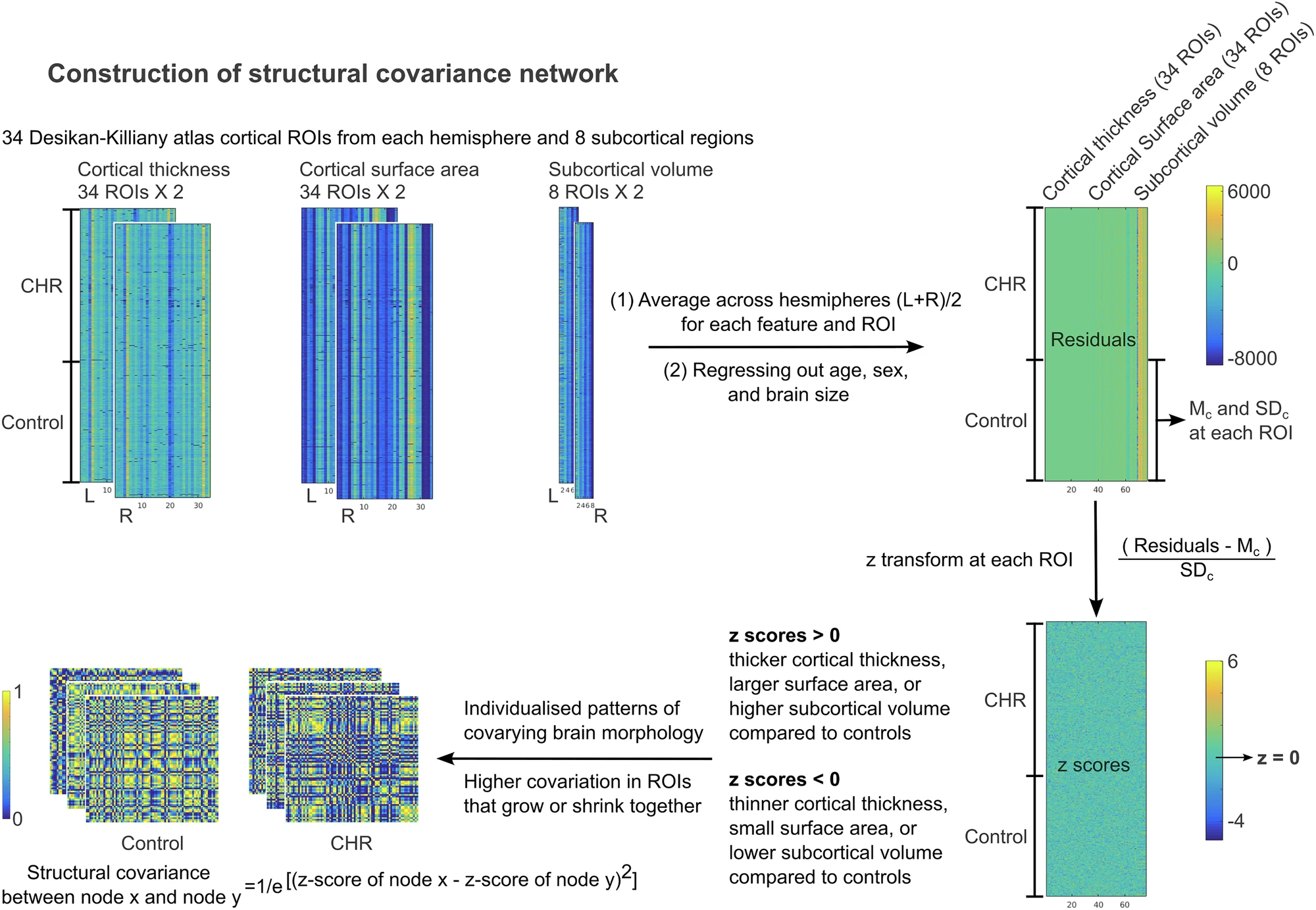
Our work builds on the ENIGMA preprocessing pipeline. T1 brain images were parcellated into 34 cortical regions per hemisphere based on Desikan-Killiany atlas and 8 subcortical regions using Freesurfer v6.0. Cortical thickness, surface area and subcortical volumes were extracted. The ENIGMA quality control protocol (https://github.com/ENIGMA-git/ENIGMA-FreeSurfer-protocol) was applied. Site and scanner-associated effects were corrected using NeuroCombat harmonisation.
Our scripts contain three sections:
- Structural covariance network construction
- Global topological properties
- Community detection and network distinctiveness
Structural covariance network construction
Structural covariance network (SCN) construction follows the methods described in Yun et al 2020 (doi: 10.1093/brain/awaa001). Steps of network construction can be found in Fig1.
Data preparation
The SCN_construction.R script was written using R software (version 4.2.1), which requirs the MASS library. It expects input data frame mydata with 159 variables (including demographic information, 3 global measures, and 152 regional values).
### example:
### 'data.frame' with 159 variables:
###  $ SID                                : Factor
###  $ Group                              : Factor with level "0" as the control group
###  $ Age                                : num
###  $ Sex                                : Factor w/ 2 levels "1_male","2_female"
###  $ LLatVent                           : num
###  $ Lthal                              : num
###  ...
###  $ RLatVent                           : num
###  $ Rthal                              : num
###  ...
###  $ L_bankssts_thickavg                : num
###  $ L_caudalanteriorcingulate_thickavg : num
###  ...
###  $ R_bankssts_thickavg                : num
###  $ R_caudalanteriorcingulate_thickavg : num
###  ...
###  $ L_bankssts_surfavg                 : num
###  $ L_caudalanteriorcingulate_surfavg  : num
###  ...
###  $ R_bankssts_surfavg                 : num
###  $ R_caudalanteriorcingulate_surfavg  : num
###  ...
###  $ ICV                         : num
###  $ TotalSA                     : num
###  $ MeanCT                      : num
You can save this data frame into a file mydata.Rdata in your working directory where all the outputs will be saved.
Running the script
- Load the data frame into the R work space.
- Source the R script so that R knows where to look for the function.
- Tell R your working directory where outputs will be saved.
- Change the directory to the working directory and run the scn function.
### example:

load('/path/to/working/directory/mydata.Rdata')

basedir='/path/to/working/directory/'

source("/path/to/script/directory/SCN_construction.R")

setwd(basedirs)
output <- scn(mydata)
mydata_hemi <- output$mydata_hemi
sc1 <- output$sc1
Several outputs are generated from this script. The mydata_hemi data frame has the regional values after standardisation. The sc1 is the structural covariance matrix. Together with the cortical and subcortical names, the mydata_hemi data frame is saved in an Rdata file with prefix output_dataframe_* and a time stamp. The script also creates a folder SC_cov1 inside the working directory, and saves the structural covariance matrix of each participant into a text file using SID as the file name.
Global topological properties
The SCN_cal_topo_S1.m, SCN_cal_topo_S2.m, and SCN_cal_PA_S3.m were tested using Matlab 2016b. An earlier version of the script was written by Zhaoping Hong (https://neuroimaginglab.org/alumni.html). The script requires adding the Graph Analysis Toolbox (GAT) toolbox, the Brain Connectivity Toolbox (BCT) toolbox, and the current script directory (so that Matlab can recognise the helper scripts in this Repository) into the Matlab path.
Running the script
- Prepare a file List.txt and include the participant IDs into a column, so that the file names inside the SC_cov1 folder can be recognised.
- Add the necessary paths to the MATLAB path.
- Run the SCN_cal_topo_S1 as a function with the necessary inputs: working directory, participant ID list, lower bound of the network sparcity threshold in percentage, and higher bound of the network sparcity threshold in percentage.
%%% example:

clear; clc;

path_to_toolbox='PATH/to/Toolbox';
scriptdir='PATH/to/scripts';
basedir='PATH/to/Working/Directory';
subjlist_file='PATH/to/Subject/List.txt';

addpath(genpath([path_to_toolbox,filesep,'GAT'])); %% adding matlab toolbox
addpath(genpath([path_to_toolbox,filesep,'BCT'])); %% adding matlab toolbox
addpath(genpath(scriptdir)); %% adding helper functions

IndMeasures = SCN_cal_topo_S1(basedir, subjlist_file,10,25); %% Here, we use top 10-25 percents as the sparcity range.
Several outputs are generated from this script. A topology folder is created to save the Matlab files. The sc_scXsubj.mat has the SCN data with SCN in rows and participant in columns. The IndMeasures variable has the thresholded data.
- Submit the SCN_cal_topo_S2 to HPC as a job. Note that most of the computations in this script should be fast. But the small-worldness index may take a few hours depending on the computational speed.
#### example:

## i, index of participants
for i in {1..100}
do

JOB=`/opt/pbs/bin/qsub -V<<EOJ
#!/bin/bash
#PBS -N "ENIGMA_$i"
#PBS -l walltime=24:00:00
#PBS -l nodes=1:ppn=1
#PBS -l mem=16gb
#PBS -e $HOME/logs/"stderr${i}.txt"
#PBS -o $HOME/logs/"stdout${i}.txt"

    module load matlab/R2016b
    matlab -nosplash -nodisplay -nodesktop -r "try; \
    path_to_toolbox='/PATH/to/toolbox/'; \
    path_to_script='/PATH/to/helper/scripts/folder/'; \
    path_to_working_directory='/PATH/to/Working/Directory/'; \
    addpath(genpath([path_to_toolbox,filesep,'GAT'])); \
    addpath(genpath([path_to_toolbox,filesep,'BCT'])); \
    addpath(genpath(path_to_script)); \
    cd(path_to_script); \
    fprintf('Running subject %d\\n'); \
    SCN_cal_topo_S2(${i}, path_to_working_directory); \
catch ME; \
    fprintf(2,'%s\\n',getReport(ME,'extended','hyperlinks','off')); \
end; exit;"

EOJ`

echo "JobID = ${JOB} submitted"

done
As an output, the IndMeasures variable has the thresholded data and the topological properties.
- Run SCN_cal_PA_S3 to calculate the area under the curve (AUC) across different sparcities. The necessary inputs include participant index, lower bound of the network sparcity threshold in percentage, higher bound of the network sparcity threshold in percentage, and the working directory.
### example: simply replace the S2 line in the step 4 job submission script above with the following line:
SCN_cal_PA_S3(${i},10,25,path_to_working_directory); \
Community detection and network distinctiveness
To identify the network architecture, we applied two-step community detection to structural covariance matrices. Using the Louvain method (https://github.com/GenLouvain/GenLouvain), we performed community detection at individual (step 1) and group (step 2) levels across sparsity levels from 10% to 25% and across gamma values from 1 to 2 at the individual level and 1 to 5 at the group level. Please ensure the GenLouvain script folder is located within the script folder.
Running the scripts
- Submit job to HPC to run the comm_detection_ind script. The necessary inputs are gamma value at the individual level, participant index, working directory, lower bound of sparcity range, and higher bound of the sparcity range.
### example:

for i in {1..2}
do

for j in {1..100}
do

JOB=`/opt/pbs/bin/qsub -V<<EOJ
#!/bin/bash
#PBS -N "EN_$j"
#PBS -l walltime=80:00:00
#PBS -l nodes=1:ppn=1
#PBS -l mem=4gb
#PBS -e $HOME/logs/"stderr${i}.txt"
#PBS -o $HOME/logs/"stdout${i}.txt"

    ##### for matlab script #####

    module load matlab/R2016b
    matlab -nosplash -nodisplay -nodesktop -r " \

    path_to_working_directory='/PATH/to/Working/Directory/'; \
    path_to_script='/PATH/to/helper/scripts/folder/'; \
    addpath(genpath(path_to_script)); \
    cd(path_to_script); \
    comm_detection_ind($i,$j,path_to_working_directory,10,25); \

    exit;" \
	############################

EOJ`

echo "JobID = ${JOB} submitted"

done
done
The outputs can be found in the newly created folder comm_det/sFC_cmodu_UNsig_R10to25/.
- Submit job to HPC to run the det_group script. The necessary inputs are gamma value at the individual level, gamma value at the group level, working directory, lower bound of sparcity range, and higher bound of the sparcity range.
### example:

for i in {1..2}
do

for j in {1..5}
do

JOB=`/opt/pbs/bin/qsub -V<<EOJ
#!/bin/bash
#PBS -N "EN_$j"
#PBS -l walltime=80:00:00
#PBS -l nodes=1:ppn=1
#PBS -l mem=4gb
#PBS -e $HOME/logs/"stderr${i}.txt"
#PBS -o $HOME/logs/"stdout${i}.txt"

    ##### for matlab script #####

    module load matlab/R2016b
    matlab -nosplash -nodisplay -nodesktop -r " \

    path_to_working_directory='/PATH/to/Working/Directory/'; \
    path_to_script='/PATH/to/helper/scripts/folder/'; \
    addpath(genpath(path_to_script)); \
    cd(path_to_script); \
    det_group($i,$j,path_to_working_directory,10,25); \

    exit;" \
	############################

EOJ`

echo "JobID = ${JOB} submitted"

done
done
The outputs can be found in the newly created folder comm_det/sFC_cmodu_UNsig_R10to25/Group/. For example, the data_gGamma2.mat file in the comm_det/sFC_cmodu_UNsig_R10to25/Group/Gamma10/ folder contains the variable CA, where the community assignments at the individual level gamma 1 and the group level gamma 2 can be found.
- Calculate the system segregation index for each community using the systemsegregation.m script (https://github.com/hzlab/2023_Chong_CommunBiol_Gripstrength_FC/blob/main/Segregation/) based on the community assignment CA.