Tensor Operations
Forward pass computes network output and “error”
Input data -> Neural Network -> Prediction
- Backward pass to compute gradients
- A fraction of the weight’s gradient is subtracted from the weight. (based on learning rate)
Neural Network <- Measure of Error
Adujst to reduce error
Learning is an Optimization Problem
-Update the weights and biases to decrease loss function
A Neural Network introductory videos with nice intutions. A 4-part series that explaines neural networks very intutively.
- 📺 What is a neural network? | Chapter 1, Deep learning
- 📺 Gradient descent, how neural networks learn | Chapter 2, Deep learning
- 📺 What is backpropagation really doing? | Chapter 3, Deep learning
- 📺 Backpropagation calculus | Chapter 4, Deep learning
Deep learning is a type of neural networks with multiple layers which can handle higher-level computation tasks, such as natural language processing, fraud detection, autonomous vehicle driving, and image recognition.
Deep learning models and their neural networks include the following:
- Convolution neural network (CNN).
- Recurrent neural network (RNN).
- Generative adversarial network (GAN).
- Autoencoder.
- Generative pre-trained transformer (GPT).
Deep Learning modeling is still an art, in other words, intelligent trial and error. There is no universal answer for NNs.
Fundamental difference in the preservation of the network state, which is absent in the feed-forward network.
GANs are a way to make generative model by having two neural network models compete each other.
| Rating | Type | Topic |
|---|---|---|
| ⭐ | 📺 | MIT Deep Learning Course - Lex Fridman |
| Rating | Type | Topic |
|---|---|---|
| ⭐ | 📺 | Nice intution about CNN, Convolutional Neural Networks |
| Rating | Type | Topic |
|---|---|---|
| ⭐ | 📺 | A friendly introduction to Recurrent Neural Networks |
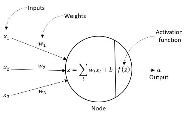
Activation functions transforms the weighted sum of a neuron so that the output is non-linear
The most common sigmoid function used in machine learning is Logistic Function, as the formula below.
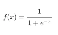
It has following properties:
- It maps the feature space into probability functions
- It uses exponential
- It is differentiable
Sigmoid function has values that are extremely near to 0 or 1. Because of this, it is appropriate for use in binary classification problems.
The Softmax function is a generalized form of the logistic function.
Softmax function has following characterstics and widely used in multi-class classification problems:
- It maps the feature space into probability functions
- It uses exponential
- It is differentiable
Softmax is used for multi-classification. The probabilities sum will be 1
References:
Think of loss function has what to minimize and optimizer how to minimize the loss.
The loss is way of measuring difference between target label(s) and prediction label(s).
- Loss could be "mean squared error", "mean absolute error loss also known as L2 Loss", "Cross Entropy" ... and in order to reduce it, weights and biases are updated after each epoch. Optimizer is used to calculate and update them.
The optimization strategies aim at minimizing the cost function.
Loss function quantifies gap between prediction and ground truth.
For regression:
- Mean Squared Error (MSE)
For classification:
- Cross Entropy Loss
Cost function and loss function are synonymous and used interchangeably, they are different.
A loss function is for a single training example. It is also sometimes called an error function. A cost function, on the other hand, is the average loss over the entire training dataset.
the log magnifies the mistake in the classification, so the misclassification will be penalized much more heavily compared to any linear loss functions. The closer the predicted value is to the opposite of the true value, the higher the loss will be, which will eventually become infinity. That’s exactly what we want a loss function to be.
when designing a neural network multi-class classifier, you can you CrossEntropyLoss with no activation, or you can use NLLLoss with log-SoftMax activation.
A good classifier will learn a decision boundary that correctly classifies most of the training data and generalizes to novel data.
Overfitting: The error decreases in the training set but increases in the test set. Overfitting example (a sine curve vs 9-degree polynomial)
Regularization
Most common regularization methods are,
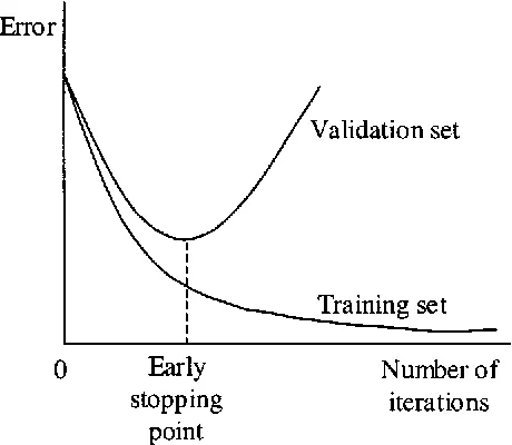
- Early Stopping - Stop training (or at least save a checkpoint) when performance on the validation set decreases. Monitor model performance on a validation set and stop training when performance degrades.
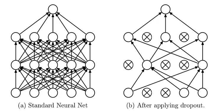
- Dropout - Randomly remove some nodes in the network (along with incoming and outgoing edges). Probabilistically remove nodes during training.
-
Usually p >= 0.5 (p is probability of keeping node)
-
Input layers p should be much higher (and use noise instead of dropout)
-
Most deep learning frameworks come with a dropout layer
-
Dropout is not used after training when making a prediction with the fit network.
- Batch Normalization (BatchNorm, BN)
- Normalize hidden layer inputs to mini-batch mean & variance
- Reduces impact of earlier layers on later layers
-
Weight Penalty (aka Weight Decay) - The simplest and perhaps most common regularization method is to add a penalty to the loss function in proportion to the size of the weights in the model. Penalize the model during training based on the magnitude of the weights.
-
Weight Constraint: Constrain the magnitude of weights to be within a range or below a limit.
-
Activity Regularization: Penalize the model during training base on the magnitude of the activations.
-
Noise: Add statistical noise to inputs during training.
Neural networks are trained by gradient descent. TDuring neural network training, stochastic gradient descent (SGD) computes the gradient of the loss functions w.r.t. its weights in the network. However, in some cases, this gradient becomes exceedingly small – hence the term “vanishing gradient.”
SGD updates a weight based on its gradient, the update is proportional to that gradient. If the gradient is vanishingly small, then the update will be vanishingly small too.
Due to this, the network learns very slowly. Also, if the adjustments are too small, the network can get stuck in a rut and stop improving altogether.
How to identify if your model suffers from a vanishing gradient problem:
- If the loss decreases very slowly over time while training.
- If you observe erratic behavior or diverging training curves.
- If the gradients in the early layer of the network are becoming increasingly small while propagating backward.
Residual connections mainly help mitigate the vanishing gradient problem.
Residual connections mainly help mitigate the vanishing gradient problem. During the back-propagation, the signal gets multiplied by the derivative of the activation function. In the case of ReLU, it means that in approximately half of the cases, the gradient is zero. Without the residual connections, a large part of the training signal would get lost during back-propagation. Residual connections reduce effect because summation is linear with respect to derivative, so each residual block also gets a signal that is not affected by the vanishing gradient. The summation operations of residual connections form a path in the computation graphs where the gradient does not get lost.
Another effect of residual connections is that the information stays local in the Transformer layer stack. The self-attention mechanism allows an arbitrary information flow in the network and thus arbitrary permuting the input tokens. The residual connections, however, always "remind" the representation of what the original state was. To some extent, the residual connections give a guarantee that contextual representations of the input tokens really represent the tokens.
A deep learning framework is said to use eager execution (or eager evaluation) if it builds its computational graph (the set of steps needed to perform forward or backwards propagation through the network) at runtime. PyTorch is the classic example of a framework which is eagerly evaluated. Every forward pass through a PyTorch model constructs an autograd computational graph; the subsequent call to backwards then consumes (and destroys!) this graph (for more on PyTorch autograd, see here).
Constructing and deconstructing objects in this way paves the way to a good developer experience. The code that’s actually executing the mathematical operations involved is ultimately a C++ or CUDA kernel, but the result of each individual operation is immediately transferred to (and accessible from) the Python process, because the Python process is the “intelligent” part—it’s what’s managing the computational graph as a whole. This is why debugging in PyTorch is as simple as dropping import pdb; pdb.set_trace() in the middle of your code.
Alternatively, one may make use of graph execution. Graph execution pushes the management of the computational graph down to the kernel level (e.g. to a C++ process) by adding an additional compilation step to the process. The state is not surfaced back to the Python process until after execution is complete.