- Describe several attention mechanisms, what are advantages and disadvantages?
- Why do we need positional encoding in transformers?
- Describe convolution types and the motivation behind them.
- How would you prevent a neural network from overfitting? How does Dropout prevent overfitting? Does it differ for train and test? How will you implement dropout during forward and backward passes?
- What is Transfer Learning? Give an example.
- What is backpropagation?
PyTorch you define your Models as subclasses of torch.nn.Module.
The init function, initializes the layers that one want to use & specify the sizes of the network.
The forward method, specifies the connections between layers.
- nn.Modules are defined as Python classes and have attributes, e.g. a
nn.Conv2dmodule will have some internal attributes likeself.weight. - nn.F.conv2d uses a functional (stateless) approach, just defines the operation and needs all arguments to be passed (including the weights and bias).
- Internally
nn.Modulesuses functional API in the forward method somewhere. - A nn.Module is actually a OO wrapper around the functional interface, that contains a number of utility methods, like eval() and parameters(), and it automatically creates the parameters of the modules for you.
- For things that do not change between training/eval like sigmoid, relu, tanh, I think it makes sense to use functional.
- torch.nn module is more used for methods which have learnable parameters. and functional for methods which do not have learnable parameters
nn.Dropout is not a trainable layer nn.Dropout changes behaviour when doing model.eval() and model.train()
All modules that make up a model may have two modes, training and test mode. These modules either have learnable parameters that need to be updated during training, like Batch Normalization or affect network topology in a sense like Dropout (by disabling some features during forward pass). some modules such as ReLU() only operate in one mode and thus do not have any change when modes change.
In .train() mode, when you feed an image, it passes trough layers until it faces a dropout and here, some features are disabled, thus their responses to the next layer is omitted, the output goes to other layers until it reaches the end of the network and you get a prediction.
the network may have correct or wrong predictions, which will accordingly update the weights. if the answer was right, the features/combinations of features that resulted in the correct answer will be positively affected and vice versa. So during training you do not need and should not disable dropout, as it affects the output and should be affecting it so that the model learns a better set of features.
In .eval() mode, before the forward pass, effectively disables all modules that has different phases for train/test mode such as Batch Normalization and Dropout (basically any module that has updateable/learnable parameters, or impacts network topology like dropout) will be disabled and you will not see them contributing to your network learning.
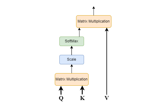
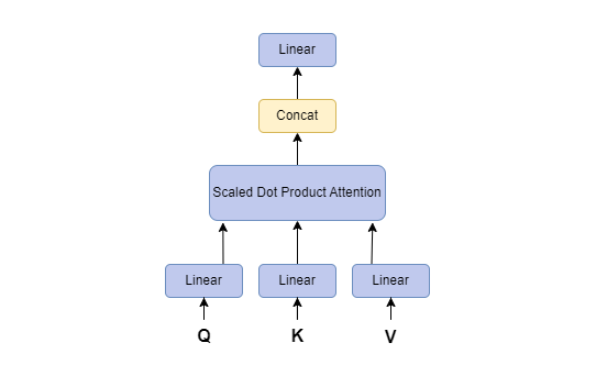
| Scaled-Dot Product Attention Mechanism | Multi-Head Attention Mechanism | Additive-Attention Mechanism | Self Attention | Entity-Aware Attention Location-Based Attention Global & Local Attentions |
|---|---|---|---|---|
| Scaled dot product is a specific formulation of multiplicative attention mechanism that calculates attention weights using dot-product of query and key vectors followed by proper scaling to prevent the dot-product from growing too large. | Instead of performing and obtaining a single Attention on large matrices Q, K and V, it is found to be more effecient to divide them into multiple matrices of smaller dimensions and perform Scaled-Dot Product on each of those smaller matrices. MultiHead attention uses multiple attention heads to attend to different parts of the input sequence which allows the model to learn different relationships between the different parts of the input sequence. For example, the model can learn to attend to the local context of a word, as well as the global context of the entire input sequence. |
This type of mechanism is used in neural networks to learn long-range dependencies between different parts of a sequence. It works by computing a weighted sum of the hidden states of the encoder, where the weights are determined by how relevant each hidden state is to the current decoding step. First, the encoder reads the input sequence and produces a sequence of hidden states which represent the encoder's understanding of the input sequence. | It is a mechanism that allows a model to attend to different parts of the same input sequence. This is done by computing a weighted sum of the input sequence, where the weights are determined by how relevant each part of the sequence is to the current task.The basic idea behind self-attention is to compute attention weights for each word/token in a sequence with respect to all other words/tokens in the same sequence. These attention weights indicate the importance or relevance of each word/token to the others. | |
 |
 |
How would you prevent a neural network from overfitting? How does Dropout prevent overfitting? Does it differ for train and test? How will you implement dropout during forward and backward passes?
Dropout is a technique to regularize in neural networks. When we drop certain nodes out, these units are not considered during a particular forward or backward pass in a network.
Dropout forces a neural network to learn more robust features that are useful in conjunction with many different random subsets of the other neurons. It will make the weights spread over the input features instead of focusing on just some features.
Dropout is used in the training phase to reduce the chance of overfitting. As you mention this layer deactivates certain neurons. The model will become more insensitive to weights of other nodes. Basically with the dropout layer the trained model will be the average of many thinned models.
The dropout will randomly mute some neurons in the neural network. At each training stage, individual nodes are either dropped out of the net
dropout is disabled in test phase.
Refer to Convolution Operations notes.
Transfer learning is a technique that involves training a model on one task, and then transferring the learned knowledge to a different, but related task. In other words, the model uses its existing knowledge to learn new tasks more efficiently.
In computer vision, transfer learning is used to fine-tune pretrained convolutional neural network (CNN) architectures like VGGNet (Simonyan & Zisserman, 2014), ResNet (He et al., 2015), the recently launched version of YOLO(v8) or Google’s* Inception Module for image classification tasks with an improved accuracy over basic CNN architectures built from scratch.
In NLP, it’s generally used to leverage pre-trained models with word embedding (vector representations of words) such as GloVe or Word2Vec.
In the realm of natural language processing (NLP), transfer learning has become increasingly popular in recent years due to the advent of large language models (LLMs), such as GPT-3 and BERT.
One of the key steps in transfer learning is the ability to freeze the layers of the pre-trained model so that only some portions of the network are updated during training. Freezing is crucial when you want to maintain the features that the pre-trained model has already learned.
Load a Pretrained Model
We’ll use the pre-trained ResNet-18 model for this example:
resnet18 = models.resnet18(pretrained=True)
Freezing Layers To freeze layers, we set the requires_grad attribute to False. This prevents PyTorch from calculating the gradients for these layers during backpropagation.
for param in resnet18.parameters():
    param.requires_grad = False
Unfreezing Some Layers
Typically, for achieving the best results, we fine-tune some fo the later layers in the network. We can do this as follows:
for param in resnet18.fc.parameters():
    param.requires_grad = True
Modifying the Network Architecture
We’ll replace the last fully-connected layer to adapt the model to a new problem with a different number of output classes (let’s say 10 classes). Also, this allows us to use this pretrained network for other applications other than classification, for example segmentation. For segmentation, we replace the final layer with a convolutional layer instead. For this example, we continue with a classification task with 10 classes.
num_ftrs = resnet18.fc.in_features
resnet18.fc = nn.Linear(num_ftrs, 10)
- The goal of backpropagation is to update the weights for the neurons in order to minimize the loss function.
- Backpropagation takes the error from the previous forward propagation and feeds this error backward through the layers to update the weights. This process is iterated until the neural network model is converged.
When building a neural network model, how do you decide what should be the architecture of your model?
Any constant initialization scheme will perform very poorly. Consider a neural network with two hidden units, and assume we initialize all the biases to 0 and the weights with some constant α. If we forward propagate an input (x1, x2) in this network, the output of both hidden units will be relu(αx1+αx2). Thus, both hidden units will have identical influence on the cost, which will lead to identical gradients. Thus, both neurons will evolve symmetrically throughout training, effectively preventing different neurons from learning different things.
if you don’t initialize your weights randomly, you will end up with some problem called the symmetry problem where every neuron is going to learn kind of the same thing. To avoid that, you will make the neuron start at different places and let them evolve independently from each other as much as possible.
Why sigmoid, Tanh is not used in hidden layers?
It results in the vanishing gradient problem and convergence will be slow towards global minima. A derivative of sigmoid lies between 0 to 0.25. A derivative of Tanh lies between 0 to 1. Because of this weight updates happen very slow.
This happens due to inappropriate weight initialization techniques. RELU works well with He initialization. Sigmoid and Tanh work well with Xavier Glorot initialization.
When you are solving binary classification use Sigmoid and when you use Multiclass classification use Softmax.
How do we decide the number of hidden layers and neurons that should be used?
- categorical_crossentropy (cce) produces a one-hot array containing the probable match for each category: [1,0,0] , [0,1,0], [0,0,1]
- sparse_categorical_crossentropy (scce) produces a category index of the most likely matching category: [1], [2], [3]
There are a number of situations to use scce, including:
- when your classes are mutually exclusive, i.e. you don’t care at all about other close-enough predictions,
- the number of categories is large to the prediction output becomes overwhelming.
Yes, CNN does perform dimensionality reduction. A pooling layer is used for this. The main objective of Pooling is to reduce the spatial dimensions of a CNN.
Deep auto-encoder
Deep residual learning is a neural network architecture that allows for training very deep networks by alleviating the vanishing gradient problem. This is done by adding “shortcut” or “skip” connections between layers in the network, which allows for information to flow more freely between layers. This makes it easier for the network to learn complex functions, and results in better performance on tasks such as image classification.

Latent space is a lower-dimensional space that captures the essential features of the input data. In simpler terms, it is a compressed representation of the original data where each dimension corresponds to a specific feature or characteristic.
Embedding vectors, or embeddings for short, encode relatively high-dimensional data into relatively low-dimensional vectors.
A fundamental property of embeddings is that they encode distance or similarity. This means that embeddings capture the semantics of the data such that similar inputs are close in the embeddings space.
Latent space is typically used synonymously with embedding space – the space into which embedding vectors are mapped.
we can think of the latent space as any feature space that contains the features, often a compressed version of the original input features.