vector.qmd

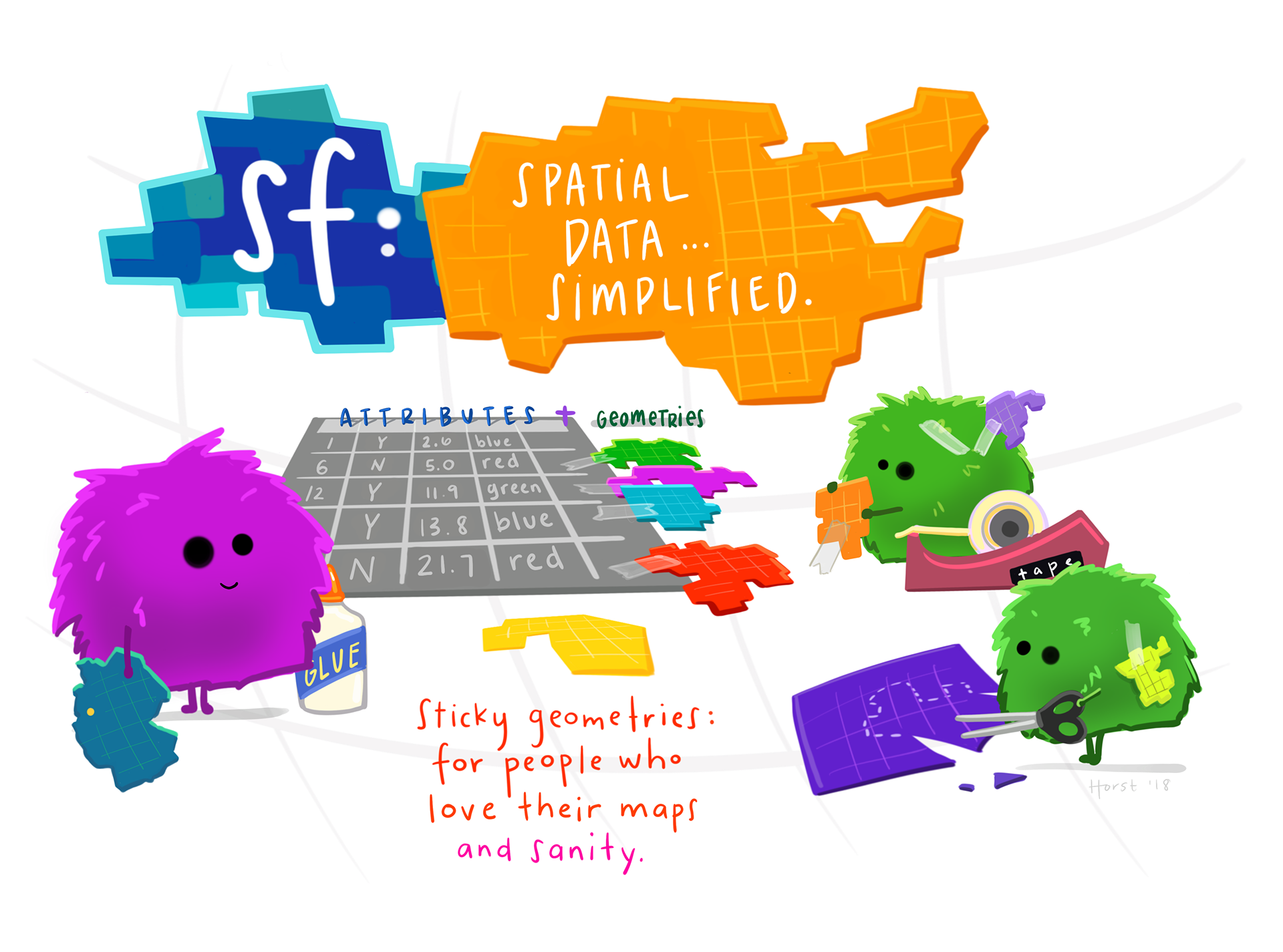
# Vector data

The first contact with spatial data is usually through vector datasets. 
Geological, hydrological, urban, and political datasets are some examples.
These datasets are usually represented by points, lines and polygons, or their derivatives.
These geometry types are represented by a hierarchical data model called the *simple features* open standard from the OGC.
In R, the simple features standard is implemented through the `sf` package [@R-sf].

```{r}
#| label: sfgeoms
#| code-fold: true
#| out-width: 70%
#| fig-cap: "Simple features supported by `sf`. Taken from [Geocomputation with R](https://r.geocompx.org/spatial-class#intro-sf)."
knitr::include_graphics("https://r.geocompx.org/figures/sf-classes.png")
```

[![](https://cdn.myportfolio.com/45214904-6a61-4e23-98d6-b140f8654a40/6025ee5a-bf25-4275-a211-16f4425089d2_rw_1920.png?h=8df287c0e9803a81d2406fdd7ff938da)]{.aside}

`sf` is the main package we focus on in this section. 
Plus, we take a look at three packages for spatial data visualisation:
`ggplot2` [@R-ggplot2], `tmap` [@R-tmap], and `mapview` [@R-mapview].

We can load them as:

```{r}
#| label: libraries
#| warning: false
library(sf)       # vector spatial data classes and functions
library(ggplot2)  # non-spatial and spatial plotting
library(tmap)     # noninteractive and interactive maps
library(mapview)  # quick interactive maps
```

## Read data into R

Reading data into R can be done from a local file or a remote file. 
If you downloaded the workshop repository, you will find the data in the `data` directory.
But, we can also fetch the data from GitHub directly, without the need to download it. 

```{r}
rivers = read_sf(
  "https://github.com/loreabad6/egu24-sc-R4geosciences/raw/main/data/nz-river-centrelines-topo-1500k.gpkg"
)
```

As you may have guessed from the object name, this is a river centreline dataset in New Zealand (Topo, 1:500k).
This data is from [Land Information New Zealand](https://data.linz.govt.nz/layer/50223-nz-river-centrelines-topo-1500k/)

We can now print the data to see how it looks like.

```{r}
rivers
```

A `sf` object shows each observation in a row and each attribute in a column.
The object header includes relevant spatial information about the object, 
like the number of rows and columns, the geometry type, dimensions, bounding box and the CRS.
Our rivers object has only one column, the geometry column.

::: {.callout-note}
You can dive deeper into sf objects and simple features in the [package documentation here](https://r-spatial.github.io/sf/articles/sf1.html).
:::

## Projections and transformations

Geographical data has a Coordinate Reference System (CRS) that allows its location on the Earth surface.
We can see the CRS of our rivers object using `sf::st_crs()` and we can easily transform the CRS using `sf::st_transform()`.

```{r}
st_crs(rivers)
st_transform(rivers, "EPSG:8857")
```

```{r}
#| layout-ncol: 2
#| fig-height: 7
#| code-fold: true
par(mar = c(0,0,2,0))
rivers |> plot(main = "EPSG: 2193")
# WGS 84 / Equal Earth Greenwich
st_transform(rivers, 8857) |> plot(main = "EPSG: 8857")
```

::: {.callout-tip}
# CRS concepts 

![](https://r-spatial.org/book/images/cover.jpg){width=25} [Section](https://r-spatial.org/book/02-Spaces.html#sec-crs) in Spatial Data Science [@stars2023] 

![](https://r.geocompx.org/images/cover.png){width=25} [Section](https://r.geocompx.org/spatial-class#crs-intro) in Geocomputation with R [@lovelace_geocomputation_2019].
:::

## Geometrical operations

Basic geometric operations such as calculating the length or area of a geometry are supported.
Let's create a new column in our data with the river length as:

```{r}
rivers["length"] = st_length(rivers)
rivers
```

To show other operations, we load another dataset.
This are administrative areas in New Zealand. 
The data comes from the `spData` package, which is a data package that has some example datasets.

```{r}
data("nz", package = "spData")
nz
summary(nz)
```

We proceed to filter our data to one of NZ regions, Gisborne. 

```{r}
(gisborne = nz[nz$Name == "Gisborne", ])
```

```{r}
#| layout-ncol: 2
#| fig-height: 7
plot(nz$geom)
plot(gisborne$geom)
```

Now, we can do operations like spatial filters and operations.
Let's try filter the river data for the Gisborne region.

[![](https://cdn.myportfolio.com/45214904-6a61-4e23-98d6-b140f8654a40/d6b4f8cb-53bf-49d5-822c-e45cd01204a4_rw_1920.png?h=9f4b33568bc02517ffe006cd7bba24f7)]{.aside}

```{r}
#| error: true
rivers |> st_intersection(gisborne)
```

That gave us an error since the data is not projected in to the same CRS. 

```{r}
gisborne = st_transform(gisborne, st_crs(rivers))
```

Let's try that again. 

```{r}
rivers |> st_intersection(gisborne)
```

We just intersected the river data with the data in the `gisborne` object.
What we are doing is an inner spatial join, where only those river linestrings that intersect the `gisborne` object stay.
Another way to do this is:

```{r}
rivers |> st_join(gisborne, left = FALSE, join = st_intersects)
```

The `join` parameter allows you to add any other type of [DE-9IM relation](https://en.wikipedia.org/wiki/DE-9IM), including your own.
So, if we want to get those river linestrings that are within the `gisborne` object we would use `sf::st_within()`. 

```{r}
rivers |> st_join(gisborne, left = FALSE, join = st_within)
```

If we don't want to do a join, that is if we don't want to bring in the columns from the second dataset, we can use `sf::st_filter()`. 
We can also specify the DE-9IM relation here with the parameter `.predicate`
```{r}
rivers |> st_filter(gisborne, .predicate = st_within)
```

This is a small plot of the difference between st_intersects and st_within.

```{r}
#| layout-ncol: 2
#| code-fold: true
par(mar = c(0,0,2,0))
int = rivers |> st_filter(gisborne, .predicate = st_intersects)
with = rivers |> st_filter(gisborne, .predicate = st_within)
plot(gisborne$geom, border = "red", col = NA, main = "st_intersects")
plot(rivers$geom, col = "grey90", alpha = 0.5, add = TRUE)
plot(int$geom, col = "blue", add = TRUE)

plot(gisborne$geom, border = "red", col = NA, main = "st_within")
plot(rivers$geom, col = "grey90", alpha = 0.5, add = TRUE)
plot(with$geom, col = "blue", add = TRUE)
```

::: {.callout-tip}
# DE-9IM concepts 

![](https://r-spatial.org/book/images/cover.jpg){width=25} [Section](https://r-spatial.org/book/03-Geometries.html#sec-de9im) in Spatial Data Science [@stars2023] 

![](https://r.geocompx.org/images/cover.png){width=25} [Section](https://r.geocompx.org/spatial-operations#DE-9IM-strings) in Geocomputation with R [@lovelace_geocomputation_2019].
:::

## Plot spatial data

Some plots have already been shown in the sections above, but let's look at this with more attention now.

### Base R

`sf` has a base plot method, which plots in small subsets the different columns of the geospatial dataset.

```{r}
plot(nz)
```

This is a great way to get a quick glance at how the data look likes.

### ggplot2

There is a `ggplot` method for sf objects, where we use the `ggplot2::geom_sf()` function to plot the sf layer.
As normal, we can call color and fill options with the data columns.
There is no need to specify any x/y coordinates since the geometry is recognised automatically.

```{r}
ggplot(nz) +
  geom_sf(aes(fill = Population))
```

::: {.callout-tip}
A great companion for making maps with {ggplot2} is [{ggspatial}](https://paleolimbot.github.io/ggspatial/index.html)!
:::

### tmap v.4

`tmap` is another option for plotting spatial features.
The package is on its way to a new version, with several breaking changes. 
Therefore, in this repository we have installed version 4 (the newer version) to showcase its usage.

```{r}
tm_shape(nz) +
  tm_fill("Name") +
  tm_shape(rivers) +
  tm_lines(col = "white", lwd = 0.7) +
  tm_scalebar()
```

### mapview

Finally, R has packages for interactive maps as well. 
While `tmap` can display some nice interactive maps, another option is `mapview`.

```{r}
mapview(nz, zcol = "Median_income")
```


::: {.callout-note}
You can find links to other R packages and resources for data visualisation [here](https://loreabad6.github.io/foss4g/slides.html).
:::

```{r}
#| include: false
# automatically create a bib database for R packages
knitr::write_bib(c(.packages()), "packages-vector.bib")
```