solution.py

# %% [markdown] tags=[]
# # Image translation (Virtual Staining)

# Written by Eduardo Hirata-Miyasaki, Ziwen Liu, and Shalin Mehta, Biohub San Francisco

# ## Overview
#
# In this exercise, we will _virtually stain_ the nuclei and plasma membrane from the quantitative phase image (QPI), i.e., translate QPI images into fluorescence images of nuclei and plasma membranes.
# QPI encodes multiple cellular structures and virtual staining decomposes these structures. After the model is trained, one only needs to acquire label-free QPI data.
# This strategy solves the same problem as "multi-spectral imaging", but is more compatible with live cell imaging and high-throughput screening.
# Virtual staining is often a step towards multiple downstream analyses: segmentation, tracking, and cell state phenotyping.
#
# In this exercise, you will:
# - Train a model to predict the fluorescence images of nuclei and plasma membranes from QPI images
# - Make it robust to variations in imaging conditions using data augmentations
# - Segment the cells using Cellpose
# - Use regression and segmentation metrics to evaluate the models
# - Visualize the image transform learned by the model
# - Understand the failure modes of the trained model
#
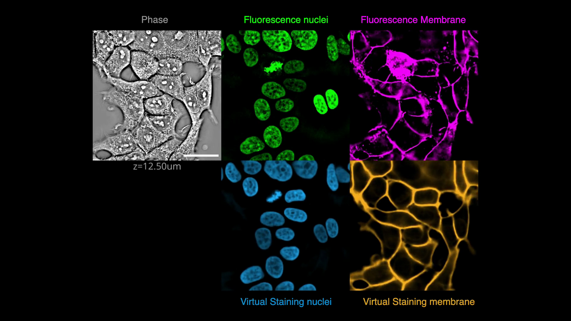# [![HEK293T](https://raw.githubusercontent.com/mehta-lab/VisCy/18d2a922ab8f41762249f9fcfff675ab8f34f32c/applications/cytoland/docs/asset/svideo_1.png)](https://github-production-user-asset-6210df.s3.amazonaws.com/67518483/343891935-d53a81eb-eb37-44f3-b522-8bd7bddc7755.mp4?X-Amz-Algorithm=AWS4-HMAC-SHA256&X-Amz-Credential=AKIAVCODYLSA53PQK4ZA%2F20260604%2Fus-east-1%2Fs3%2Faws4_request&X-Amz-Date=20260604T191111Z&X-Amz-Expires=300&X-Amz-Signature=7cbe992928146b9284ed045c9a8e8fc5e18d59308dddbfcbb26362c653ebd0b2&X-Amz-SignedHeaders=host&response-content-type=video%2Fmp4)
# (Click on image to play video)
#
# %% [markdown] tags=[]
# ### Goals

# #### Part 1: Train a virtual staining model
#
#   - Explore OME-Zarr using [iohub](https://czbiohub-sf.github.io/iohub/main/index.html)
#   and the high-content-screen (HCS) format.
#   - Use our `viscy.data.HCSDataloader()` dataloader and explore the  3 channel (phase, fluorescence nuclei and cell membrane)
#   A549 cell dataset.
#   - Implement data augmentations [MONAI](https://monai.io/) to train a robust model to imaging parameters and conditions.
#   - Use tensorboard to log the augmentations, training and validation losses and batches
#   - Start the training of the UNeXt2 model to predict nuclei and membrane from phase images.
#
# #### Part 2: Evaluate the model to translate phase into fluorescence.
#   - Compare the performance of your trained model with the _VSCyto2D_ pre-trained model.
#   - Evaluate the model using pixel-level and instance-level metrics.
#
# #### Part 3: Visualize the image transforms learned by the model and explore the model's regime of validity
#   - Visualize the first 3 principal components mapped to a color space in each encoder and decoder block.
#   - Explore the model's regime of validity by applying blurring and scaling transforms to the input phase image.
#
# #### For more information:
# Checkout [VisCy](https://github.com/mehta-lab/VisCy),
# our deep learning pipeline for training and deploying computer vision models
# for image-based phenotyping including the robust virtual staining of landmark organelles.
#
# VisCy exploits recent advances in data and metadata formats
# ([OME-zarr](https://link.springer.com/article/10.1007/s00418-023-02209-1)) and DL frameworks,
# [PyTorch Lightning](https://lightning.ai/) and [MONAI](https://monai.io/).

# ### References
# - [Liu, Z. and Hirata-Miyasaki, E. et al. (2025) Robust virtual staining of landmark organelles with Cytoland](https://www.nature.com/articles/s42256-025-01046-2)
# - [Guo et al. (2020) Revealing architectural order with quantitative label-free imaging and deep learning. eLife](https://elifesciences.org/articles/55502)

# %% [markdown] tags=[]
# <div class="alert alert-success">
# The exercise is organized in 3 parts:

# <ul>
# <li><b>Part 1</b> - Train a virtual staining model using iohub (I/O library), VisCy dataloaders, and tensorboard</li>
# <li><b>Part 2</b> - Evaluate the model to translate phase into fluorescence.</li>
# <li><b>Part 3</b> - Visualize the image transforms learned by the model and explore the model's regime of validity.</li>
# </ul>

# </div>

# %% [markdown] tags=[]
# <div class="alert alert-danger">
# Set your python kernel to <span style="color:black;">04_image_translation</span>
# </div>

# %% [markdown] tags=[]
# ## PyTorch Lightning Intro
#
# If you've used plain PyTorch you already know the pattern: write a model, write a
# `for batch in dataloader` loop, move tensors to `cuda`, call `loss.backward()`, step
# the optimizer, remember to `zero_grad()`, log every N steps, save a checkpoint, and
# repeat for validation. That boilerplate is the same in every project — so
# [PyTorch Lightning](https://lightning.ai) factors it out into **three objects** and
# owns the training loop for you.
#
# | Lightning object | What it holds | In this exercise |
# | --- | --- | --- |
# | `LightningDataModule` | How to load, split, augment, and batch your data (`train/val/test/predict_dataloader`) | `HCSDataModule` — reads OME-Zarr and yields `{"source": ..., "target": ...}` dicts |
# | `LightningModule` | The network, the loss, and what happens in `training_step` / `validation_step` (one batch at a time) | `VSUNet` — wraps the UNeXt2 architecture and the virtual-staining loss |
# | `Trainer` | The loop: device placement, mixed precision, logging, checkpointing, multi-GPU | `VisCyTrainer` — a thin subclass with VisCy-friendly defaults |
#
# You don't write a `for` loop. You call **`trainer.fit(model, datamodule)`** and
# Lightning drives everything. The trainer handles:
#
# - moving batches to the right device (`accelerator="gpu"`, `devices=[0]`)
# - mixed-precision training (`precision="16-mixed"`) so you use less GPU memory
# - when to log metrics / images (`log_every_n_steps`) and where (`logger=TensorBoardLogger(...)`)
# - saving checkpoints automatically under the logger's directory
# - running a sanity check on a single batch before real training (`fast_dev_run=True`)
#
# VisCy builds on top of Lightning and provides the `HCSDataModule` and `VSUNet`
# classes so you don't have to subclass `LightningDataModule` / `LightningModule`
# yourself. You configure them via constructor arguments and let Lightning run.
# When you see `trainer.fit(...)` below, that single call replaces a ~50-line hand-
# written training loop.

# %% [markdown]
# # Part 1: Log training data to tensorboard, start training a model.
# ---------
# Learning goals:

# - Load the OME-zarr dataset and examine the channels (A549).
# - Configure and understand the data loader.
# - Log some patches to tensorboard.
# - Initialize a 2D UNeXt2 model for virtual staining of nuclei and membrane from phase.
# - Start training the model to predict nuclei and membrane from phase.

# %% Imports
import os
from glob import glob
from pathlib import Path
from typing import Tuple

import matplotlib.pyplot as plt
import numpy as np
import pandas as pd
import torch
import torchview
from cellpose import models
from cmap import Colormap
from iohub import open_ome_zarr
from iohub.reader import print_info
from lightning.pytorch import seed_everything
from lightning.pytorch.loggers import TensorBoardLogger

from skimage.metrics import structural_similarity
from natsort import natsorted
from numpy.typing import ArrayLike

# pytorch lightning wrapper for Tensorboard.
from skimage.color import label2rgb
from torch.utils.tensorboard import SummaryWriter  # for logging to tensorboard
from torchmetrics.functional import accuracy, jaccard_index
from torchmetrics.functional.segmentation import dice_score
from tqdm import tqdm

# Trainer class and UNet from the cytoland package.
from cytoland.engine import VSUNet

# HCSDataModule makes it easy to load data during training.
from viscy_data.hcs import HCSDataModule

# training augmentations
from viscy_transforms import (
    CenterSpatialCropd,
    NormalizeSampled,
    RandAdjustContrastd,
    RandAffined,
    RandGaussianNoised,
    RandGaussianSmoothd,
    RandScaleIntensityd,
    RandWeightedCropd,
)
from viscy_utils.evaluation.metrics import mean_average_precision
from viscy_utils.losses import MixedLoss
from viscy_utils.trainer import VisCyTrainer

# %%
# seed random number generators for reproducibility.
seed_everything(42, workers=True)

# %% tags=["task"]
# Set the path to the data.
#
# `top_dir` is the folder that contains training/, test/, and
# pretrained_models/. On the course machines the data is staged at
# /mnt/efs/dl_jrc/data/04_image_translation, so you can leave this as is.
#
# #######################
# ##### TODO ########
# #######################
top_dir = Path("/mnt/efs/dl_jrc/data/04_image_translation")

# %% tags=["solution"]
# `top_dir` points directly at the data folder (training/, test/,
# pretrained_models/).
# #######################
# ##### SOLUTION ########
# #######################
top_dir = Path("/mnt/efs/dl_jrc/data/04_image_translation")

# %%
# Derived paths. `top_dir` must point at the folder containing training/,
# test/, and pretrained_models/.
data_path = top_dir / "training/a549_hoechst_cellmask_train_val.zarr"

# Path where we will save our training logs
training_top_dir = Path(f"{os.getcwd()}/data/")
# Create top_training_dir directory if needed, and launch tensorboard
training_top_dir.mkdir(parents=True, exist_ok=True)
log_dir = training_top_dir / "04_image_translation/logs/"
# Create log directory if needed, and launch tensorboard
log_dir.mkdir(parents=True, exist_ok=True)

if not data_path.exists():
    raise FileNotFoundError(
        f"Data not found at {data_path}. Please check the top_dir and data_path variables."
    )

# %% [markdown] tags=[]
# The next cell starts tensorboard.

# <div class="alert alert-warning">
# If you launched jupyter lab from ssh terminal, add <code>--host &lt;your-server-name&gt;</code> to the tensorboard command below. <code>&lt;your-server-name&gt;</code> is the address of your compute node that ends in amazonaws.com.

# </div>


# %%  tags=[]
# Visualization and TensorBoard helpers (live in utils.py to keep this
# notebook focused on the machine learning content). Open utils.py if you
# want to see how each helper renders its inputs.
from utils import (
    BOP_BLUE,
    BOP_ORANGE,
    GREEN,
    MAGENTA,
    clip_highlight,
    clip_p,
    composite_nuc_mem,
    launch_tensorboard,
    log_batch_jupyter,
    log_batch_tensorboard,
    process_image,
)


# Launch tensorboard and click on the link to view the logs.
tensorboard_process = launch_tensorboard(log_dir)
# %% [markdown] tags = []
# <div class="alert alert-warning">
# If you are using VSCode and a remote server, you will need to forward the port to view the tensorboard. <br>
# Take note of the port number was assigned in the previous cell.(i.e <code> http://localhost:{port_number_assigned}</code>) <br>

# Locate the your VSCode terminal and select the <code>Ports</code> tab <br>
# <ul>
# <li>Add a new port with the <code>port_number_assigned</code>
# </ul>
# Click on the link to view the tensorboard and it should open in your browser.
# </div>


# %% [markdown] tags=[]
# ## Load OME-Zarr Dataset
#
# **OME-Zarr** is a chunked, cloud-friendly microscopy format; **HCS layout**
# nests the zarr store like a physical plate — `row/col/field/level/T/C/Z/Y/X` —
# so each FOV is addressable by `dataset[f"{row}/{col}/{field}/{level}"]` and
# returns an `(T, C, Z, Y, X)` array.
#
# This dataset has 24 FOVs of 2048×2048 images across 3 channels (QPI, nuclei
# stained with DAPI, membrane stained with Cellmask), four pyramid levels
# (`0` = 2048×2048, `1` = 1024×1024, `2` = 512×512, `3` = 256×256), and a single
# time point. Pyramid levels let you preview a whole FOV cheaply at low
# resolution before zooming in to full resolution for training/inference.

# %% [markdown]
# ![OME-Zarr HCS layout](https://media.springernature.com/lw685/springer-static/image/art%3A10.1007%2Fs00418-023-02209-1/MediaObjects/418_2023_2209_Fig2_HTML.png)
#
# *Figure 2 from Moore et al. (2023), "OME-Zarr: a cloud-optimized bioimaging
# file format with international community support", Histochemistry and Cell
# Biology. Reproduced under [CC BY 4.0](https://creativecommons.org/licenses/by/4.0/).
# Article: https://link.springer.com/article/10.1007/s00418-023-02209-1*

# %% [markdown] tags=[]
# <div class="alert alert-warning">
# You can inspect the tree structure by using your terminal:
# <code> iohub info -v "path-to-ome-zarr" </code>

# <br>
# More info on the CLI:
# <code>iohub info --help </code> to see the help menu.
# </div>
# %%
# This is the python function called by `iohub info` CLI command
print_info(data_path, verbose=True)

# Open and inspect the dataset.
dataset = open_ome_zarr(data_path)

# %% [markdown] tags=[]
# <div class="alert alert-info">
#
# ### Task 1.1
# Look at a couple different fields of view (FOVs) by changing the `field` variable.
# Check the cell density, the cell morphologies, and fluorescence signal.
# HINT: look at the HCS Plate format to see what your options are.
# </div>
# %% tags=[]
# Use the field below to visualize data. Pyramid levels are shown side-by-side
# (0 = full resolution, larger = downsampled previews).
row = 0
col = 0
field = 9  # TODO: Change this to explore data.

# `channel_names` is the metadata that is stored with data according to the OME-NGFF spec.
n_channels = len(dataset.channel_names)

# Per-channel colormaps for the standard fluorescence-microscopy convention:
# phase as grayscale, nuclei in green, membrane in magenta.
channel_cmaps = {
    "Phase3D": Colormap("gray").to_mpl(),
    "Nucl": Colormap("green").to_mpl(),
    "Mem": Colormap("magenta").to_mpl(),
}
default_cmap = Colormap("gray").to_mpl()

# Enumerate the pyramid levels for this FOV via iohub's Position.images().
# Each level is the same FOV downsampled (2048 -> 1024 -> 512 -> 256 in YX),
# not a smaller crop of the full-resolution data.
position = dataset[f"{row}/{col}/{field}"]
pyramid_levels = [(path, arr) for path, arr in position.images()]
print(f"FOV: {field}, pyramid levels: {[p for p, _ in pyramid_levels]}")

figure, axes = plt.subplots(
    len(pyramid_levels),
    n_channels,
    figsize=(n_channels * 3, len(pyramid_levels) * 3),
    squeeze=False,
)

for level_idx, (level_path, level_arr) in enumerate(pyramid_levels):
    image = np.asarray(level_arr)
    print(f"  level {level_path}: shape={image.shape}")
    for ch_idx in range(n_channels):
        # Display the central z-slice so every level uses the same focal plane.
        z_index = image.shape[2] // 2
        channel_image = image[0, ch_idx, z_index]
        # Adjust contrast to 0.5th and 99.5th percentile of pixel values.
        p_low, p_high = np.percentile(channel_image, (0.5, 99.5))
        channel_image = np.clip(channel_image, p_low, p_high)
        ax = axes[level_idx, ch_idx]
        ax.imshow(
            channel_image,
            cmap=channel_cmaps.get(dataset.channel_names[ch_idx], default_cmap),
        )
        ax.axis("off")
        ax.set_title(
            f"{dataset.channel_names[ch_idx]} — level {level_path} "
            f"({channel_image.shape[0]}×{channel_image.shape[1]})"
        )
plt.tight_layout()

# %% [markdown] tags=[]
# ## Explore the effects of augmentation on batch.
#
# Time to meet the first of the three Lightning objects from the primer above: the
# **DataModule**. `HCSDataModule` is VisCy's `LightningDataModule` — it knows how
# to read an OME-Zarr store, split FOVs into train/val, apply normalization and
# augmentations, and hand the Trainer a PyTorch `DataLoader`. You configure it
# once; Lightning calls the right method (`train_dataloader()`,
# `val_dataloader()`, etc.) at the right time.
#
# Every sample `HCSDataModule` yields is a Python `dict` (not a tuple) with:
#
# - `source`: the input image, a tensor of shape `(1, 1, Y, X)` → `(C, Z, Y, X)`
# - `target`: the target image, a tensor of shape `(2, 1, Y, X)` → `(C, Z, Y, X)`
# - `index` : the tuple `(HCS location, time, z-slice)` identifying the sample
#
# A `batch` is a dict of the same keys with an extra leading batch dimension, e.g.
# `batch["source"].shape == (B, 1, 1, Y, X)`. The `training_step` method inside
# `VSUNet` receives this dict directly — no unpacking required.

# %% [markdown] tags=[]
# ## A primer on augmentations and patch sizes
#
# You pass augmentations to `HCSDataModule` via the `augmentations=[...]`
# argument. They run on the **CPU**, inside each `DataLoader` worker, per
# sample, before the batch is collated and moved to the GPU. The chain runs in
# order, so the *last* transform in the list determines the final patch size
# the model sees.
#
# Two things to keep in mind when designing the chain:
#
# 1. **Some augmentations work better on a larger crop than the model's final
#    input size.** A common pattern is "crop to 384×384, rotate, then
#    center-crop to 256×256" — that way the rotation's black corners get
#    cropped out before the model sees the patch. So you'll often want
#    `RandWeightedCropd` (e.g. 384×384) → spatial / intensity transforms →
#    `CenterSpatialCropd` (e.g. 256×256) at the end of the chain.
# 2. **`HCSDataModule` validates the final patch size.** Right before each
#    training batch hits the model, it checks that the source spatial shape
#    matches `(z_window_size, *yx_patch_size)`. If it doesn't, you'll get a
#    `ValueError` telling you to add a spatial crop. Practically: whatever the
#    last spatial-sizing transform produces must equal `yx_patch_size`.
#
# (Advanced: the data module also supports a `gpu_augmentations=[...]`
# argument that runs per-batch on the GPU after `on_after_batch_transfer`.
# We don't use it in this exercise — keeping everything CPU-side is simpler
# and is enough for this dataset.)

# %% [markdown] tags=[]
# <div class="alert alert-info">
#
# ### Task 1.2
# - Run the next cell to setup a logger for your augmentations.
# - Setup the `HCSDataloader()` in for training.
#   - Configure the dataloader for the `"UNeXt2_2D"`
#   - Configure the dataloader for the phase (source) to fluorescence cell nuclei and membrane (targets) regression task.
#   - Configure the dataloader for training. Hint: use the `HCSDataloader.setup()`
# - Open your tensorboard and look at the `IMAGES tab`.
#
# Note: If tensorboard is not showing images or the plots, try refreshing and using the "Images" tab.
# </div>


# %% tags=["task"]
# Initialize the data module.

BATCH_SIZE = 16

# 4 is a perfectly reasonable batch size
# (batch size does not have to be a power of 2)
# See: https://sebastianraschka.com/blog/2022/batch-size-2.html

# #######################
# ##### TODO ########
# #######################
# HINT: Run dataset.channel_names
source_channel = ["TODO"]
target_channel = ["TODO", "TODO"]

# #######################
# ##### TODO ########
# #######################
data_module = HCSDataModule(
    data_path,
    z_window_size=1,
    source_channel=source_channel,
    target_channel=target_channel,
    split_ratio=0.8,
    batch_size=BATCH_SIZE,
    num_workers=4,
    yx_patch_size=(256, 256),  # larger patch size makes it easy to see augmentations.
    # Crop to yx_patch_size so the visualization batch is 256x256, not the
    # full 2048x2048 FOV — otherwise this single un-augmented batch would
    # pin several GB of GPU memory through the rest of the notebook.
    # No random augmentations yet (rotations / noise / contrast come in
    # Task 1.3).
    augmentations=[
        CenterSpatialCropd(
            keys=source_channel + target_channel,
            roi_size=(1, 256, 256),
        ),
    ],
    normalizations=[],  # Turn off normalization for now.
)
# #######################
# ##### TODO  ########
# #######################
# Setup the data_module to fit. HINT: data_module.setup()


# Evaluate the data module
print(
    f"Samples in training set: {len(data_module.train_dataset)}, "
    f"samples in validation set:{len(data_module.val_dataset)}"
)
train_dataloader = data_module.train_dataloader()
# Instantiate the tensorboard SummaryWriter, logs the first batch and then iterates through all the batches and logs them to tensorboard.
writer = SummaryWriter(log_dir=f"{log_dir}/view_batch")
# Draw a batch and write to tensorboard.
batch = next(iter(train_dataloader))
log_batch_tensorboard(batch, 0, writer, "augmentation/none")
writer.close()
# %% tags=["solution"]

BATCH_SIZE = 16
# 4 is a perfectly reasonable batch size
# (batch size does not have to be a power of 2)
# See: https://sebastianraschka.com/blog/2022/batch-size-2.html

# #######################
# ##### SOLUTION ########
# #######################
source_channel = ["Phase3D"]
target_channel = ["Nucl", "Mem"]

# #######################
# ##### SOLUTION ########
# #######################
data_module = HCSDataModule(
    data_path,
    z_window_size=1,
    source_channel=source_channel,
    target_channel=target_channel,
    split_ratio=0.8,
    batch_size=BATCH_SIZE,
    num_workers=4,
    yx_patch_size=(256, 256),  # larger patch size makes it easy to see augmentations.
    # Crop to yx_patch_size so the visualization batch is 256x256, not the
    # full 2048x2048 FOV — otherwise this single un-augmented batch would
    # pin several GB of GPU memory through the rest of the notebook.
    # No random augmentations yet (rotations / noise / contrast come in
    # Task 1.3).
    augmentations=[
        CenterSpatialCropd(
            keys=source_channel + target_channel,
            roi_size=(1, 256, 256),
        ),
    ],
    normalizations=[],  # Turn off normalization for now.
)

# #######################
# ##### SOLUTION ########
# #######################
# Setup the data_module to fit. HINT: data_module.setup()
data_module.setup("fit")

# Evaluate the data module
print(
    f"Samples in training set: {len(data_module.train_dataset)}, "
    f"samples in validation set:{len(data_module.val_dataset)}"
)
train_dataloader = data_module.train_dataloader()
# Instantiate the tensorboard SummaryWriter, logs the first batch and then iterates through all the batches and logs them to tensorboard.
writer = SummaryWriter(log_dir=f"{log_dir}/view_batch")
# Draw a batch and write to tensorboard.
batch = next(iter(train_dataloader))
log_batch_tensorboard(batch, 0, writer, "augmentation/none")
writer.close()
# %% [markdown] tags=[]
# <div class="alert alert-warning">
#
# ### Questions
# 1. What are the two channels in the target image?
# 2. How many samples are in the training and validation set? What determined that split?
#
# Note: If tensorboard is not showing images, try refreshing and using the "Images" tab.
# </div>

# %% [markdown] tags=[]
# If your tensorboard is causing issues, you can visualize directly on Jupyter /VSCode
# %%
# Visualize in Jupyter
log_batch_jupyter(batch, dataset.channel_names)

# %% [markdown] tags=[]
# <div class="alert alert-warning">
# <h3> Question for Task 1.3 </h3>
# 1. How do they make the model more robust to imaging parameters or conditions
# without having to acquire data for every possible condition? <br>
# </div>
# %% [markdown] tags=["solution"]
# Each augmentation simulates a real-world source of microscope-to-microscope
# variation so the model doesn't overfit to the training conditions:
#
# | Transform | Simulates |
# | --- | --- |
# | `RandWeightedCropd` | random crops biased toward signal-dense regions (foreground oversampling) |
# | `RandAffined` | stage rotation, scale drift, slight shear between acquisitions |
# | `RandAdjustContrastd` | illumination / exposure differences |
# | `RandScaleIntensityd` | gain / brightness differences between cameras |
# | `RandGaussianNoised` | shot and read noise at different detector settings |
# | `RandGaussianSmoothd` | small focus drift / defocus |
# %% [markdown] tags=[]
# <div class="alert alert-info">
#
# ### Task 1.3
# Add the following augmentations:
# - Add augmentations to rotate about $\pi$ around z-axis, 30% scale in (y,x),
# shearing of 1% in (y,x), and no padding with zeros with a probability of 80%.
# - Add a Gaussian noise with a mean of 0.0 and standard deviation of 0.3 with a probability of 50%.
#
# HINT: `RandAffined()` and `RandGaussianNoised()` are MONAI dictionary
# transforms re-exported from `viscy_transforms`. See the MONAI docs for
# arguments and probability semantics:
# [RandAffined](https://docs.monai.io/en/stable/transforms.html#randaffined),
# [RandGaussianNoised](https://docs.monai.io/en/stable/transforms.html#randgaussiannoised).
# You can also inspect any transform in a cell with `RandAffined?`.<br><br>
# [Compare your choice of augmentations against the pretrained models and config files](https://github.com/mehta-lab/VisCy/releases/download/v0.1.0/VisCy-0.1.0-VS-models.zip).
#
# <br><br>
# <b>Question:</b> Once you run the next cell, notice the black corners
# in the rotated patches. Where do they come from, and how can you make
# sure the model never sees them? (Hint: look at the
# <code>padding_mode</code> kwarg in <code>RandAffined</code>, and compare
# the patch size you visualize here with <code>yx_patch_size</code>. The
# last transform in the augmentation chain determines what the model
# actually receives — what should that transform be?)
# </div>
# %% tags=["task"]
# Here we turn on data augmentation and rerun setup
# #######################
# ##### TODO ########
# #######################
# HINT: Run dataset.channel_names
source_channel = ["TODO"]
target_channel = ["TODO", "TODO"]

augmentations = [
    RandWeightedCropd(
        keys=source_channel + target_channel,
        spatial_size=(1, 384, 384),
        num_samples=2,
        w_key=target_channel[0],
    ),
    # #######################
    # ##### TODO  ########
    # #######################
    ## TODO: Add Random Affine Transorms
    ## Write code below
    # #######################
    RandAdjustContrastd(keys=source_channel, prob=0.5, gamma=(0.8, 1.2)),
    RandScaleIntensityd(keys=source_channel, factors=0.5, prob=0.5),
    # #######################
    # ##### TODO  ########
    # #######################
    ## TODO: Add Random Gaussian Noise
    ## Write code below
    # #######################
    RandGaussianSmoothd(
        keys=source_channel,
        sigma_x=(0.25, 0.75),
        sigma_y=(0.25, 0.75),
        sigma_z=(0.0, 0.0),
        prob=0.5,
    ),
    # #######################
    # ##### TODO  ########
    # #######################
    ## TODO: Add a CenterSpatialCropd
    ## Write code below
    # #######################
]

normalizations = [
    NormalizeSampled(
        keys=source_channel,
        level="fov_statistics",
        subtrahend="mean",
        divisor="std",
    ),
    NormalizeSampled(
        keys=target_channel,
        level="fov_statistics",
        subtrahend="median",
        divisor="iqr",
    ),
]

data_module.augmentations = augmentations
data_module.normalizations = normalizations

data_module.setup("fit")

# get the new data loader with augmentation turned on
augmented_train_dataloader = data_module.train_dataloader()

# Draw batches and write to tensorboard
writer = SummaryWriter(log_dir=f"{log_dir}/view_batch")
augmented_batch = next(iter(augmented_train_dataloader))
log_batch_tensorboard(augmented_batch, 0, writer, "augmentation/some")
writer.close()

# %% tags=["solution"]
# #######################
# ##### SOLUTION ########
# #######################
source_channel = ["Phase3D"]
target_channel = ["Nucl", "Mem"]

augmentations = [
    RandWeightedCropd(
        keys=source_channel + target_channel,
        spatial_size=(1, 384, 384),
        num_samples=2,
        w_key=target_channel[0],
    ),
    # #######################
    # ##### SOLUTION ########
    # #######################
    RandAffined(
        keys=source_channel + target_channel,
        rotate_range=[3.14, 0.0, 0.0],
        scale_range=[0.0, 0.3, 0.3],
        prob=0.8,
        padding_mode="zeros",
        shear_range=[0.0, 0.01, 0.01],
    ),
    RandAdjustContrastd(keys=source_channel, prob=0.5, gamma=(0.8, 1.2)),
    RandScaleIntensityd(keys=source_channel, factors=0.5, prob=0.5),
    # #######################
    # ##### SOLUTION ########
    # #######################
    RandGaussianNoised(keys=source_channel, prob=0.5, mean=0.0, std=0.3),
    RandGaussianSmoothd(
        keys=source_channel,
        sigma_x=(0.25, 0.75),
        sigma_y=(0.25, 0.75),
        sigma_z=(0.0, 0.0),
        prob=0.5,
    ),
    # #######################
    # ##### SOLUTION ########
    # #######################
    # Final center crop down to yx_patch_size. The rotated 384x384 patch has
    # black corners from RandAffined's zero padding; cropping to the central
    # 256x256 removes them before the patch reaches the model. Without this
    # last step HCSDataModule raises a ValueError in on_after_batch_transfer.
    CenterSpatialCropd(
        keys=source_channel + target_channel,
        roi_size=(1, 256, 256),
    ),
]

normalizations = [
    NormalizeSampled(
        keys=source_channel,
        level="fov_statistics",
        subtrahend="mean",
        divisor="std",
    ),
    NormalizeSampled(
        keys=target_channel,
        level="fov_statistics",
        subtrahend="median",
        divisor="iqr",
    ),
]

data_module.augmentations = augmentations

# Setup the data_module to fit. HINT: data_module.setup()
data_module.setup("fit")

# get the new data loader with augmentation turned on
augmented_train_dataloader = data_module.train_dataloader()

# Draw batches and write to tensorboard
writer = SummaryWriter(log_dir=f"{log_dir}/view_batch")
augmented_batch = next(iter(augmented_train_dataloader))
log_batch_tensorboard(augmented_batch, 0, writer, "augmentation/some")
writer.close()

# %% [markdown] tags=[]
# <div class="alert alert-warning">
# <h3> Question for Task 1.3 </h3>
# 1. Look at your tensorboard. Can you tell the agumentations were applied to the sample batch? Compare the batch with and without augmentations. <br>
# 2. Are these augmentations good enough? What else would you add?
# </div>

# %% [markdown]
# Visualize directly on Jupyter

# %%
log_batch_jupyter(augmented_batch, dataset.channel_names)

# %% [markdown] tags=[]
# ## Train a 2D U-Net model to predict nuclei and membrane from phase.
# ### Constructing a 2D UNeXt2 using VisCy
#
# Now we meet the second Lightning object: the **`LightningModule`**. `VSUNet` is
# VisCy's `LightningModule` and it bundles three things that plain PyTorch keeps
# separate:
#
# 1. **The network** — a UNeXt2 architecture, configured through `model_config`.
# 2. **The loss** — passed in as `loss_function=MixedLoss(...)`. VisCy's
#    `MixedLoss` is a single class with knobs for L1, L2/MSE, and MS-DSSIM.
#    For this exercise we'll train with pure MSE (`l2_alpha=1.0`); the
#    pretrained checkpoint we compare against in Part 2 was trained with
#    a mix of L1 + MS-DSSIM.
# 3. **The per-batch logic** — `training_step` and `validation_step` methods that
#    take one `{"source", "target"}` batch, run the forward pass, compute the
#    loss, and return it. You don't see these methods here because they're
#    defined once inside `VSUNet`; Lightning calls them for you.
#
# Other constructor arguments you'll recognize from plain PyTorch training:
# `lr` is the learning rate, `schedule="WarmupCosine"` picks the LR schedule,
# and `freeze_encoder=False` lets gradients flow through the whole network.
# `log_batches_per_epoch` is a VisCy extra — it tells the module how many image
# samples to push to TensorBoard each epoch.
# %% [markdown]
# **Architecture config** — UNeXt2 is a U-Net with ConvNeXt-style blocks:
#
# - `encoder_blocks=[3, 3, 9, 3]` and `dims=[96, 192, 384, 768]` — 4 downsampling
#   stages with that many blocks and feature channels per stage (last stage is
#   the bottleneck). More blocks / dims = more capacity and more compute.
# - `decoder_conv_blocks=2` — conv blocks after each upsampling step.
# - `stem_kernel_size=(1, 2, 2)` and `in_stack_depth=1` — this is a 2D model,
#   so we use 1 z-slice and a stem that doesn't convolve across z.
#
# **Loss** — `MixedLoss(l2_alpha=1.0)` is plain MSE (mean squared error) on
# the predicted vs target fluorescence — the most familiar regression loss,
# and a good baseline for image translation.
#
# Once your model trains, try swapping the loss with
# `MixedLoss(l1_alpha=0.5, ms_dssim_alpha=0.5)` (per-pixel L1 + multi-scale
# SSIM). L1 + MS-DSSIM is what the pretrained VSCyto2D checkpoint we
# compare against in Part 2 was trained with, and produces visibly sharper
# membrane edges than MSE alone.
#
# **Schedule** — `schedule="WarmupCosine"`, `lr=6e-4`: the learning rate ramps
# up from 0 over the first few epochs (warmup), then follows a cosine decay
# toward 0. Warmup lets AdamW's adaptive step-size estimates stabilize before
# taking large steps, preventing early training instability; cosine decay is a
# strong default for vision transformer / ConvNeXt-style encoders.

# %% [markdown]
# <div class="alert alert-info">
#
# ### Task 1.4
# - Run the next cell to instantiate the `UNeXt2_2D` model
#   - Configure the network for the phase (source) to fluorescence cell nuclei and membrane (targets) regression task.
#   - Call the VSUNet with the `"UNeXt2_2D"` architecture.
# - Run the next cells to instantiate data module and trainer.
#   - Add the source channel name and the target channel names
# - Start the training <br>
#
# <b> Note </b> <br>
# See ``viscy.translation.engine.VSUNet`` ([source code](https://github.com/mehta-lab/VisCy/blob/main/viscy/translation/engine.py)) and ``viscy.unet.networks.fcmae`` ([source code](https://github.com/mehta-lab/VisCy/blob/main/viscy/unet/networks/fcmae.py)) to learn more about the configuration parameters and FCMAE architecture.
# </div>

# %% tags=["task"]
# Create a 2D UNet.
GPU_ID = 0

BATCH_SIZE = 16
YX_PATCH_SIZE = (256, 256)

# #######################
# ##### TODO ########
# #######################
# Dictionary that specifies key parameters of the model.
phase2fluor_config = dict(
    in_channels=...,  # TODO how many input channels are we feeding Hint: int?,
    out_channels=...,  # TODO how many output channels are we solving for? Hint: int,
    encoder_blocks=[3, 3, 9, 3],
    dims=[96, 192, 384, 768],
    decoder_conv_blocks=2,
    stem_kernel_size=(1, 2, 2),
    in_stack_depth=...,  # TODO: was this a 2D or 3D input? HINT: int,
    pretraining=False,
)

# #######################
# ##### TODO ########
# #######################
phase2fluor_model = VSUNet(
    architecture=...,  # TODO: 2D UNeXt2 architecture
    model_config=phase2fluor_config.copy(),
    loss_function=MixedLoss(l1_alpha=0.0, l2_alpha=1.0, ms_dssim_alpha=0.0),
    schedule="WarmupCosine",
    lr=6e-4,
    log_batches_per_epoch=5,  # Number of samples from each batch to log to tensorboard.
    freeze_encoder=False,
)

# #######################
# ##### TODO ########
# #######################
# HINT: Run dataset.channel_names
source_channel = ["TODO"]
target_channel = ["TODO", "TODO"]

# Setup the data module.
# NOTE: the `augmentations` chain you build above must end with a
# CenterSpatialCropd that brings patches down to yx_patch_size. HCSDataModule
# validates this and will raise ValueError if the
# final source shape doesn't match the model's expected input shape.
phase2fluor_2D_data = HCSDataModule(
    data_path,
    source_channel=source_channel,
    target_channel=target_channel,
    z_window_size=1,
    split_ratio=0.8,
    batch_size=BATCH_SIZE,
    num_workers=4,
    yx_patch_size=YX_PATCH_SIZE,
    augmentations=augmentations,
    val_augmentations=[
        CenterSpatialCropd(
            keys=source_channel + target_channel,
            roi_size=(1, YX_PATCH_SIZE[0], YX_PATCH_SIZE[1]),
        ),
    ],
    normalizations=normalizations,
)
phase2fluor_2D_data.setup("fit")


# fast_dev_run runs a single batch of data through the model to check for errors.
trainer = VisCyTrainer(
    accelerator="gpu", devices=[GPU_ID], precision="16-mixed", fast_dev_run=True
)

# trainer class takes the model and the data module as inputs.
trainer.fit(phase2fluor_model, datamodule=phase2fluor_2D_data)


# %% tags=["solution"]

# Here we are creating a 2D UNet.
GPU_ID = 0

BATCH_SIZE = 16
YX_PATCH_SIZE = (256, 256)

# Dictionary that specifies key parameters of the model.
# #######################
# ##### SOLUTION ########
# #######################
phase2fluor_config = dict(
    in_channels=1,
    out_channels=2,
    encoder_blocks=[3, 3, 9, 3],
    dims=[96, 192, 384, 768],
    decoder_conv_blocks=2,
    stem_kernel_size=(1, 2, 2),
    in_stack_depth=1,
    pretraining=False,
)

phase2fluor_model = VSUNet(
    architecture="UNeXt2_2D",  # 2D UNeXt2 architecture
    model_config=phase2fluor_config.copy(),
    loss_function=MixedLoss(l1_alpha=0.0, l2_alpha=1.0, ms_dssim_alpha=0.0),
    schedule="WarmupCosine",
    lr=6e-4,
    log_batches_per_epoch=5,  # Number of samples from each batch to log to tensorboard.
    freeze_encoder=False,
)

# ### Instantiate data module and trainer, test that we are setup to launch training.
# #######################
# ##### SOLUTION ########
# #######################
# Selecting the source and target channel names from the dataset.
source_channel = ["Phase3D"]
target_channel = ["Nucl", "Mem"]
# Setup the data module.
# NOTE: the `augmentations` chain above ends with a CenterSpatialCropd that
# brings patches down to yx_patch_size before the batch reaches the model.
# HCSDataModule validates this in on_after_batch_transfer.
phase2fluor_2D_data = HCSDataModule(
    data_path,
    source_channel=source_channel,
    target_channel=target_channel,
    z_window_size=1,
    split_ratio=0.8,
    batch_size=BATCH_SIZE,
    num_workers=4,
    yx_patch_size=YX_PATCH_SIZE,
    augmentations=augmentations,
    val_augmentations=[
        CenterSpatialCropd(
            keys=source_channel + target_channel,
            roi_size=(1, YX_PATCH_SIZE[0], YX_PATCH_SIZE[1]),
        ),
    ],
    normalizations=normalizations,
)
# #######################
# ##### SOLUTION ########
# #######################
phase2fluor_2D_data.setup("fit")

# --- The third Lightning object: the Trainer ---
#
# This is the object that replaces the hand-written training loop. Each kwarg
# controls one piece of the boilerplate Lightning is handling for you:
#
# - accelerator="gpu", devices=[GPU_ID]
#       Pick the device. No more ".to(device)" sprinkled through your code —
#       Lightning moves model + every batch for you.
# - precision="16-mixed"
#       Automatic mixed-precision training (fp16 activations, fp32 master
#       weights). Cuts GPU memory roughly in half and speeds up matmuls on
#       modern GPUs — no autocast() context managers needed.
# - fast_dev_run=True
#       Sanity check: run ONE training batch + ONE validation batch and exit.
#       Use this on every new pipeline to catch shape bugs, NaN losses, or
#       bad paths *before* you commit to a multi-hour training job.
#
# trainer.fit(model, datamodule=...) then drives the whole thing: it calls
# datamodule.setup(), pulls batches from train_dataloader(), invokes
# model.training_step(batch), runs loss.backward() + optimizer.step() +
# zero_grad(), runs validation, logs to TensorBoard, and saves checkpoints.
trainer = VisCyTrainer(
    accelerator="gpu", devices=[GPU_ID], precision="16-mixed", fast_dev_run=True
)
trainer.fit(phase2fluor_model, datamodule=phase2fluor_2D_data)

# %% [markdown] tags=[]
# ## View model graph.
#
# PyTorch uses dynamic graphs under the hood.
# The graphs are constructed on the fly.
# This is in contrast to TensorFlow,
# where the graph is constructed before the training loop and remains static.
# In other words, the graph of the network can change with every forward pass.
# Therefore, we need to supply an input tensor to construct the graph.
# NOTE: The input tensor can be a random tensor of the correct shape and type.
# We can also supply a real image from the dataset.
# The latter is more useful for debugging.

# %% [markdown]
# <div class="alert alert-info">
#
# ### Task 1.5
# Run the next cell to generate a graph representation of the model architecture.
# </div>

# %%
# Visualize graph of phase2fluor model as image.
#
# RandWeightedCropd(num_samples=2) makes train_dataset[i]["source"] a list of
# 2 crops, so we can't just call .unsqueeze on it. We feed torchview a dummy
# tensor of the model's expected input shape directly:
# (B, C, Z, Y, X) = (1, 1, 1, 256, 256).
dummy_input = torch.zeros(
    1, 1, 1, YX_PATCH_SIZE[0], YX_PATCH_SIZE[1], dtype=torch.float32
)
model_graph_phase2fluor = torchview.draw_graph(
    phase2fluor_model,
    dummy_input,
    roll=True,
    depth=3,  # adjust depth to zoom in.
    device="cpu",
    # expand_nested=True,
)
# Print the image of the model.
model_graph_phase2fluor.visual_graph

# %% [markdown] tags=[]
# <div class="alert alert-warning">
#
# ### Question:
# Can you recognize the UNet structure and skip connections in this graph visualization?
# </div>

# %% [markdown]
# <div class="alert alert-info">

# <h3> Task 1.6 </h3>
# Start training by running the following cell. Check the new logs on the tensorboard.
# </div>

# %% [markdown]
# Now that `fast_dev_run` confirmed the pipeline works end-to-end, we switch
# to a "real" Trainer configured for an actual multi-epoch run. New Lightning
# knobs appearing here:
#
# - `max_epochs=n_epochs` — run this many passes over the training set, then stop.
# - `log_every_n_steps=steps_per_epoch // 2` — how often Lightning flushes
#   scalars (loss, learning rate) to the logger. Setting it to half an epoch
#   gives us two data points per epoch without spamming TensorBoard.
# - `logger=TensorBoardLogger(save_dir=log_dir, name="phase2fluor", log_graph=True)`
#   — Lightning writes TensorBoard event files *and* model checkpoints under
#   `{save_dir}/{name}/version_N/`. You don't call `torch.save` yourself; the
#   trainer persists checkpoints automatically, and `log_graph=True` adds the
#   network architecture to the Graphs tab.
#
# Calling `trainer.fit` again below runs the full training loop — forward,
# loss, backward, optimizer step, validation every epoch, checkpoint at the
# end — across `max_epochs` epochs.

# %% tags=["task"]
# Check if GPU is available
# You can check by typing `nvidia-smi`
GPU_ID = 0

n_samples = len(phase2fluor_2D_data.train_dataset)
steps_per_epoch = n_samples // BATCH_SIZE  # steps per epoch.

# #######################
# ##### TODO ########
# #######################
# How many passes over the training set should we run? Pick a value
# (20-30 is a reasonable starting point on the course AWS T4 GPUs —
# each epoch is ~0.5 min, so ~10-15 min total). You can monitor training
# progress in TensorBoard
n_epochs = ...  # TODO

trainer = VisCyTrainer(
    accelerator="gpu",
    devices=[GPU_ID],
    max_epochs=n_epochs,
    precision="16-mixed",
    log_every_n_steps=steps_per_epoch // 2,
    # log losses and image samples 2 times per epoch.
    logger=TensorBoardLogger(
        save_dir=log_dir,
        # lightning trainer transparently saves logs and model checkpoints in this directory.
        name="phase2fluor",
        log_graph=True,
    ),
)
# Launch training and check that loss and images are being logged on tensorboard.
trainer.fit(phase2fluor_model, datamodule=phase2fluor_2D_data)

# Move the model to the GPU.
device = torch.device("cuda" if torch.cuda.is_available() else "cpu")
phase2fluor_model.to(device)

# %% tags=["solution"]
GPU_ID = 0

n_samples = len(phase2fluor_2D_data.train_dataset)
steps_per_epoch = n_samples // BATCH_SIZE
# #######################
# ##### SOLUTION ########
# #######################
n_epochs = 30

trainer = VisCyTrainer(
    accelerator="gpu",
    devices=[GPU_ID],
    max_epochs=n_epochs,
    precision="16-mixed",
    log_every_n_steps=steps_per_epoch // 2,
    logger=TensorBoardLogger(
        save_dir=log_dir,
        name="phase2fluor",
        log_graph=True,
    ),
)
trainer.fit(phase2fluor_model, datamodule=phase2fluor_2D_data)

device = torch.device("cuda" if torch.cuda.is_available() else "cpu")
phase2fluor_model.to(device)
# %% [markdown] tags=[]
# <div class="alert alert-success">

# <h2> Checkpoint 1 </h2>

# While your model is training, let's think about the following questions:<br>
# <ul>
# <li>What is the information content of each channel in the dataset?</li>
# <li>How would you use image translation models?</li>
# <li>What can you try to improve the performance of each model?</li>
# </ul>

# Now the training has started,
# we can come back after a while and evaluate the performance!

# </div>
# %% [markdown] tags=[]
# # Part 2: Assess your trained model
#
# We evaluate on a held-out test set using two complementary families of metrics:
#
# - **Regression / pixel-level** (Pearson, SSIM): are predicted
#   intensities close to ground truth, per pixel? Cheap, but can hide
#   topological errors — a model that merges two nuclei may still score well
#   pixel-wise.
# - **Segmentation / instance-level** (Jaccard/IoU, Dice, mAP over IoU
#   thresholds): run Cellpose on both predicted and measured fluorescence,
#   then compare instance masks. This is what ultimately matters for
#   downstream analysis (counting cells, tracking, phenotyping).
#
# Also inspect the validation samples on TensorBoard — the experimental
# nuclei channel is noisy, so "ground truth" is itself imperfect.

# %% [markdown]
# <div class="alert alert-info">

# <h3> Task 2.1 Define metrics </h3>

# For each of the above metrics, write a brief definition of what they are and what they mean
# for this image translation task. Use your favorite search engine and/or resources.

# </div>

# %% [markdown] tags=["solution"]
# **Solution — metric definitions:**
#
# - **Pearson Correlation**: linear correlation between predicted and target
#   intensities across all pixels, in `[-1, 1]`. `1` means the prediction is a
#   perfect affine rescaling of the target; invariant to mean / contrast
#   offsets. Good at flagging "the pattern is right" but blind to structural
#   errors that preserve correlation (e.g. a uniformly blurred prediction).
#
# - **SSIM ([Structural Similarity](https://en.wikipedia.org/wiki/Structural_similarity))**:
#   patch-wise compares local mean, variance, and covariance between
#   prediction and target. It captures structure Pearson misses — blurring,
#   contrast loss, edge softness. We use
#   `skimage.metrics.structural_similarity` with `data_range=1` after
#   normalizing both arrays to `[0, 1]`. Note: SSIM was designed for
#   natural images; on sparse, low-dynamic-range microscopy data it tends
#   to compress into a narrow band, so treat absolute SSIM values as
#   relative to other models on the same task, not as universal quality
#   numbers.

# %% [markdown] tags=[]
# ### Let's compute metrics directly and plot below.
# %% [markdown] tags=[]
# <div class="alert alert-danger">
# If you weren't able to train or training didn't complete please run the following lines to load the latest checkpoint <br>
#
# ```python
# phase2fluor_model_ckpt = natsorted(glob(
#    str(training_top_dir / "04_image_translation/logs/phase2fluor/version*/checkpoints/*.ckpt")
# ))[-1]
# ```
# <br>
# NOTE: if their model didn't go past epoch 5, lost their checkpoint, or didnt train anything.
# Run the following:
#
# ```python
# phase2fluor_model_ckpt = natsorted(glob(
#  str(top_dir/"04_image_translation/pretrained_models/backup/version_10/checkpoints/*.ckpt")
# ))[-1]
# ```

# ```python
# phase2fluor_config = dict(
#     in_channels=1,
#     out_channels=2,
#     encoder_blocks=[3, 3, 9, 3],
#     dims=[96, 192, 384, 768],
#     decoder_conv_blocks=2,
#     stem_kernel_size=(1, 2, 2),
#     in_stack_depth=1,
#     pretraining=False,
# )
#
# phase2fluor_model = VSUNet.load_from_checkpoint( #Load the model checkpoint
#     phase2fluor_model_ckpt,
#     architecture="UNeXt2_2D",
#     model_config = phase2fluor_config,
#     accelerator='gpu'
# )
# ````
# </div>
# %%
# Setup the test data module.
test_data_path = top_dir / "test/a549_hoechst_cellmask_test.zarr"
source_channel = ["Phase3D"]
target_channel = ["Nucl", "Mem"]

test_data = HCSDataModule(
    test_data_path,
    source_channel=source_channel,
    target_channel=target_channel,
    z_window_size=1,
    batch_size=1,
    num_workers=4,
    normalizations=[
        NormalizeSampled(
            keys=source_channel,
            level="fov_statistics",
            subtrahend="mean",
            divisor="std",
        ),
        NormalizeSampled(
            keys=target_channel,
            level="fov_statistics",
            subtrahend="median",
            divisor="iqr",
        ),
    ],
)
test_data.setup("test")

test_metrics = pd.DataFrame(
    columns=["pearson_nuc", "SSIM_nuc", "pearson_mem", "SSIM_mem"]
)


# %%
# Compute metrics directly and plot here.
#
# Two helpers:
#   normalize_fov  -> z-score (zero mean, unit variance), used to put the
#                     phase *input* in the same statistical range the model
#                     was trained on.
#   min_max_scale  -> [0, 1] range, used to put the *target* and *prediction*
#                     into a known dynamic range before passing them to SSIM
#                     (so `data_range=1` is exactly correct).
def normalize_fov(input: ArrayLike):
    "Normalize an FOV to zero mean and unit variance (used for model input)."
    mean = np.mean(input)
    std = np.std(input)
    return (input - mean) / std


def min_max_scale(image: ArrayLike) -> ArrayLike:
    "Rescale an image to the [0, 1] range (used before SSIM)."
    min_val = image.min()
    max_val = image.max()
    dynamic_range = max_val - min_val
    if dynamic_range <= np.finfo(float).eps:
        return np.zeros_like(image, dtype=float)
    return (image - min_val) / dynamic_range


for i, sample in enumerate(
    tqdm(test_data.test_dataloader(), desc="Computing metrics per sample")
):
    phase_image = sample["source"].to(phase2fluor_model.device)
    with torch.inference_mode():  # turn off gradient computation.
        predicted_image = phase2fluor_model(phase_image)

    target_image = (
        sample["target"].cpu().numpy().squeeze(0)
    )  # Squeezing batch dimension.
    predicted_image = predicted_image.cpu().numpy().squeeze(0)
    phase_image = phase_image.cpu().numpy().squeeze(0)
    # Rescale target + prediction to [0, 1] so SSIM's `data_range=1` is
    # exactly the dynamic range of the arrays we pass in.
    target_mem = min_max_scale(target_image[1, 0, :, :])
    target_nuc = min_max_scale(target_image[0, 0, :, :])
    # slicing channel dimension, squeezing z-dimension.
    predicted_mem = min_max_scale(predicted_image[1, :, :, :].squeeze(0))
    predicted_nuc = min_max_scale(predicted_image[0, :, :, :].squeeze(0))

    # Compute SSIM and pearson correlation.
    ssim_nuc = structural_similarity(target_nuc, predicted_nuc, data_range=1)
    ssim_mem = structural_similarity(target_mem, predicted_mem, data_range=1)
    pearson_nuc = np.corrcoef(target_nuc.flatten(), predicted_nuc.flatten())[0, 1]
    pearson_mem = np.corrcoef(target_mem.flatten(), predicted_mem.flatten())[0, 1]

    test_metrics.loc[i] = {
        "pearson_nuc": pearson_nuc,
        "SSIM_nuc": ssim_nuc,
        "pearson_mem": pearson_mem,
        "SSIM_mem": ssim_mem,
    }

# Plot the following metrics
test_metrics.boxplot(
    column=["pearson_nuc", "SSIM_nuc", "pearson_mem", "SSIM_mem"],
    rot=30,
)


# %%
# Plot the predicted image vs target image.
# Layout: 2 rows x 3 columns — phase input on the left, ground truth
# (real fluorescence) on the top row, virtual staining (prediction) on
# the bottom row. Eye-friendly side-by-side comparison.
fig, axes = plt.subplots(2, 3, figsize=(18, 12))

for i, sample in enumerate(test_data.test_dataloader()):
    phase_image = sample["source"]

    with torch.inference_mode():  # turn off gradient computation.
        predicted_image = (
            phase2fluor_model(phase_image.to(phase2fluor_model.device))
            .cpu()
            .numpy()
            .squeeze(0)
        )

    target_image = sample["target"].cpu().numpy().squeeze(0)
    phase_raw = process_image(phase_image[0, 0, 0])
    predicted_nuclei = process_image(predicted_image[0, 0])
    predicted_membrane = process_image(predicted_image[1, 0])
    target_nuclei = process_image(target_image[0, 0])
    target_membrane = process_image(target_image[1, 0])

    # Row 0: input phase, target nuclei (real), target membrane (real)
    axes[0, 0].imshow(phase_raw, cmap="gray")
    axes[0, 0].set_title("Phase (input)")
    axes[0, 1].imshow(target_nuclei, cmap="gray")
    axes[0, 1].set_title("Nuclei — fluorescence (target)")
    axes[0, 2].imshow(target_membrane, cmap="gray")
    axes[0, 2].set_title("Membrane — fluorescence (target)")

    # Row 1: blank under phase, predicted nuclei, predicted membrane
    axes[1, 0].axis("off")
    axes[1, 1].imshow(predicted_nuclei, cmap="gray")
    axes[1, 1].set_title("Nuclei — virtual staining (predicted)")
    axes[1, 2].imshow(predicted_membrane, cmap="gray")
    axes[1, 2].set_title("Membrane — virtual staining (predicted)")

    for ax in axes.flat:
        ax.axis("off")
    plt.tight_layout()
    plt.show()
    break
# %% [markdown] tags=[]
# <div class="alert alert-info">

# <h3> Task 2.2 Loading the pretrained model VSCyto2D </h3>
# Here we will compare your model with the VSCyto2D pretrained model by computing the pixel-based metrics and segmentation-based metrics.
#
# <ul>
# <li>The pretrained checkpoint was downloaded by <code>setup.sh</code> to
#   <code>/mnt/efs/dl_jrc/data/04_image_translation/pretrained_models/VSCyto2D/epoch=399-step=23200.ckpt</code>
#   — if missing, download it directly from
#   <a href="https://public.czbiohub.org/comp.micro/viscy/VS_models/VSCyto2D/VSCyto2D/epoch=399-step=23200.ckpt">public.czbiohub.org</a>.
#   Check with <code>ls /mnt/efs/dl_jrc/data/04_image_translation/pretrained_models/VSCyto2D/</code>.</li>
# <li>Load the <b>VSCyto2D</b> model checkpoint and the configuration file</li>
# <li>Compute the pixel-based metrics and segmentation-based metrics between the model you trained and the pretrained model</li>
# </ul>
# <br>

# </div>


# %% tags=["task"]
#################
##### TODO ######
#################
# Let's load the pretrained model checkpoint
pretrained_model_ckpt = (
    top_dir / ...
)  ## Add the path to the "VSCyto2D/epoch=399-step=23200.ckpt"

# TODO: Load the phase2fluor_config just like the model you trained in Task 1.4.
# HINT: copy the dict you built above verbatim — same in_channels, out_channels,
# encoder_blocks, dims, decoder_conv_blocks, stem_kernel_size, in_stack_depth.
phase2fluor_config = dict(
    in_channels=...,  # TODO: same as Task 1.4
    out_channels=...,  # TODO: same as Task 1.4
    encoder_blocks=...,  # TODO: same as Task 1.4
    dims=...,  # TODO: same as Task 1.4
    decoder_conv_blocks=...,  # TODO: same as Task 1.4
    stem_kernel_size=...,  # TODO: same as Task 1.4
    in_stack_depth=...,  # TODO: same as Task 1.4
    pretraining=False,
)

# TODO: Load the checkpoint. Write the architecture name. HINT: look at the previous config.
pretrained_phase2fluor = VSUNet.load_from_checkpoint(
    pretrained_model_ckpt,
    architecture=...,
    model_config=phase2fluor_config,
)
# Move the loaded model to GPU (VSUNet does not take an accelerator kwarg;
# Lightning's trainer handles that for fit/predict, but for manual inference
# we move the module ourselves).
pretrained_phase2fluor = pretrained_phase2fluor.to(
    torch.device(f"cuda:{GPU_ID}" if torch.cuda.is_available() else "cpu")
)
# TODO: Setup the dataloader in evaluation/predict mode
#

# %% tags=["solution"]
# #######################
# ##### SOLUTION ########
# #######################

pretrained_model_ckpt = top_dir / "pretrained_models/VSCyto2D/epoch=399-step=23200.ckpt"

phase2fluor_config = dict(
    in_channels=1,
    out_channels=2,
    encoder_blocks=[3, 3, 9, 3],
    dims=[96, 192, 384, 768],
    decoder_conv_blocks=2,
    stem_kernel_size=(1, 2, 2),
    in_stack_depth=1,
    pretraining=False,
)
# Load the model checkpoint
device = torch.device("cuda" if torch.cuda.is_available() else "cpu")
pretrained_phase2fluor = VSUNet.load_from_checkpoint(
    pretrained_model_ckpt,
    architecture="UNeXt2_2D",
    model_config=phase2fluor_config,
    map_location=device,
)
pretrained_phase2fluor = pretrained_phase2fluor.to(device)
pretrained_phase2fluor.eval()

### Re-load your trained model
# NOTE: assuming the latest checkpoint it your latest training and model
phase2fluor_model_ckpt = natsorted(
    glob(
        str(
            training_top_dir
            / "04_image_translation/logs/phase2fluor/version*/checkpoints/*.ckpt"
        )
    )
)[-1]

# NOTE: if their model didn't go past epoch 5, lost their checkpoint, or didnt train anything.
# Uncomment the next lines
# phase2fluor_model_ckpt = natsorted(glob(
#  str(training_top_dir/"04_image_translation/backup/phase2fluor/version_0/checkpoints/*.ckpt")
# ))[-1]

phase2fluor_config = dict(
    in_channels=1,
    out_channels=2,
    encoder_blocks=[3, 3, 9, 3],
    dims=[96, 192, 384, 768],
    decoder_conv_blocks=2,
    stem_kernel_size=(1, 2, 2),
    in_stack_depth=1,
    pretraining=False,
)
# Load the model checkpoint, then move it to GPU for manual inference.
# (VSUNet does not accept an accelerator kwarg — Lightning's Trainer handles
# device placement automatically for fit/predict, but here we call the model
# directly, so we move it explicitly.)
phase2fluor_model = VSUNet.load_from_checkpoint(
    phase2fluor_model_ckpt,
    architecture="UNeXt2_2D",
    model_config=phase2fluor_config,
).to(torch.device(f"cuda:{GPU_ID}" if torch.cuda.is_available() else "cpu"))
phase2fluor_model.eval()
# %% [markdown] tags=[]
# <div class="alert alert-warning">
# <h3> Question </h3>
# 1. Can we evaluate a model's performance based on their segmentations?<br>
# 2. Look up IoU or Jaccard index, dice coefficient, and AP metrics. LINK:https://metrics-reloaded.dkfz.de/metric-library <br>
# We will evaluate the performance of your trained model with a pre-trained model using pixel based metrics as above and
# segmantation based metrics including (mAP@0.5, dice, accuracy and jaccard index). <br>
# </div>
# %% [markdown] tags=["solution"]
#
# - <b> IoU (Intersection over Union): </b> Also referred to as the Jaccard index, is essentially a method to quantify the percent overlap between the target and predicted masks.
# It is calculated as the intersection of the target and predicted masks divided by the union of the target and predicted masks. <br>
# - <b> Dice Coefficient:</b> Metric used to evaluate the similarity between two sets.<br>
# It is calculated as twice the intersection of the target and predicted masks divided by the sum of the target and predicted masks.<br>
# - <b> mAP (mean Average Precision):</b>  The mean Average Precision (mAP) is a metric used to evaluate the performance of object detection models.
# It is calculated as the average precision across all classes and is used to measure the accuracy of the model in localizing objects.
#
# %% [markdown] tags=[]
# ### Let's compute the metrics for the test dataset
# Before you run the following code, make sure you have the pretrained model loaded and the test data is ready.

# The following code will compute the following:
# - the pixel-based metrics  (pearson correlation, SSIM)
# - segmentation-based metrics (mAP@0.5, dice, accuracy, jaccard index)


# #### Note:
# - The segmentation-based metrics are computed using the cellpose stock `nuclei` model
# - The metrics will be store in the `test_pixel_metrics` and `test_segmentation_metrics` dataframes
# - The segmentations will be stored in the `segmentation_store` zarr file
# - Analyze the code while it runs.
# %%
# Create cellpose model once for reuse
device = torch.device("cuda" if torch.cuda.is_available() else "cpu")
cellpose_model = models.CellposeModel(
    gpu=True if device.type == "cuda" else False, device=device
)


# Define the function to compute the cellpose segmentation
def cellpose_segmentation(
    prediction: ArrayLike, target: ArrayLike
) -> Tuple[torch.ShortTensor]:
    # NOTE these are hardcoded for this notebook and A549 dataset

    # Convert 2D arrays to 3D format expected by cellpose v4.0.1+
    # Add channel dimension and replicate to 3 channels (RGB format)
    if prediction.ndim == 2:
        prediction = np.tile(prediction, (3, 1, 1))  # Shape: (3, H, W)
    if target.ndim == 2:
        target = np.tile(target, (3, 1, 1))  # Shape: (3, H, W)

    cp_nuc_kwargs = {
        "diameter": 65,
        "cellprob_threshold": 0.0,
    }

    # Batch prediction and target into a single Cellpose call so they share
    # one GPU forward pass instead of two — roughly halves runtime per call.
    masks_list, _, _ = cellpose_model.eval([prediction, target], **cp_nuc_kwargs)
    pred_label, target_label = masks_list

    pred_label = pred_label.astype(np.int32)
    target_label = target_label.astype(np.int32)
    pred_label = torch.ShortTensor(pred_label)
    target_label = torch.ShortTensor(target_label)

    return (pred_label, target_label)


# %%
# Setting the paths for the test data and the output segmentation
test_data_path = top_dir / "test/a549_hoechst_cellmask_test.zarr"
output_segmentation_path = (
    training_top_dir / "04_image_translation/pretrained_model_segmentations.zarr"
)

# Creating the dataframes to store the pixel and segmentation metrics
test_pixel_metrics = pd.DataFrame(
    columns=[
        "model",
        "fov",
        "pearson_nuc",
        "SSIM_nuc",
        "pearson_mem",
        "SSIM_mem",
    ]
)
test_segmentation_metrics = pd.DataFrame(
    columns=[
        "model",
        "fov",
        "masks_per_fov",
        "accuracy",
        "dice",
        "jaccard",
        "mAP",
        "mAP_50",
        "mAP_75",
        "mAR_100",
    ]
)
# Opening the test dataset
test_dataset = open_ome_zarr(test_data_path)

# Looking at the test dataset
print("Test dataset:")
test_dataset.print_tree()
channel_names = test_dataset.channel_names
print(f"Channel names: {channel_names}")

# Finding the channel indices for the corresponding channel names
phase_cidx = channel_names.index("Phase3D")
nuc_cidx = channel_names.index("Nucl")
mem_cidx = channel_names.index("Mem")
nuc_label_cidx = channel_names.index("nuclei_segmentation")


# %% [markdown]
# ## Visualize segmentation comparison: Fluorescence vs Virtual Staining vs Pretrained
# Let's compare nucleus and membrane segmentation across all three models

# %%
# Compare real fluorescence vs virtual staining (trained & pretrained models),
# with Cellpose segmentation, on a 300x300 center crop of one test FOV.
positions = list(test_dataset.positions())  # reused by the metrics cell below
fov, sample_pos = positions[0]  # use the first FOV as example

T, C, Z, Y, X = sample_pos.data.shape
z = Z // 2
crop = 300
ys, xs = Y // 2 - crop // 2, X // 2 - crop // 2
sl = (slice(ys, ys + crop), slice(xs, xs + crop))  # center-crop selector

# Phase input MUST be normalized the same way the models were trained
# (per-FOV z-score, same as `normalize_fov` used in the metrics cell). Without
# this the predictions collapse into a faint copy of the phase image.
phase = normalize_fov(sample_pos.data[0, phase_cidx, z].astype(np.float32))
phase_tensor = torch.from_numpy(phase)[None, None, None].to(device)  # (B, C, Z, Y, X)


def virtual_stain(model):
    """Predict (nucleus, membrane), center-cropped and min-max scaled for display."""
    with torch.inference_mode():
        nuc, mem = model(phase_tensor).cpu().numpy()[0, :, 0]  # (2, Y, X)
    return min_max_scale(nuc[sl]), min_max_scale(mem[sl])


# The three conditions to compare, each a (nucleus, membrane) image pair.
conditions = {
    "Fluorescence": (
        min_max_scale(sample_pos.data[0, nuc_cidx, z][sl].astype(np.float32)),
        min_max_scale(sample_pos.data[0, mem_cidx, z][sl].astype(np.float32)),
    ),
    "Virtual (trained)": virtual_stain(phase2fluor_model),
    "Virtual (pretrained)": virtual_stain(pretrained_phase2fluor),
}

# rows = conditions, cols = nucleus | nucleus-seg | membrane | membrane-seg
fig, axes = plt.subplots(3, 4, figsize=(16, 12))
counts = {}
for row, (name, (nuc_img, mem_img)) in enumerate(conditions.items()):
    nuc_seg = cellpose_segmentation(nuc_img, nuc_img)[0].numpy()
    mem_seg = cellpose_segmentation(mem_img, mem_img)[0].numpy()
    counts[name] = (len(np.unique(nuc_seg)) - 1, len(np.unique(mem_seg)) - 1)
    panels = [
        (nuc_img, "gray", f"{name}\nNucleus"),
        (label2rgb(nuc_seg, nuc_img, bg_label=0), None, "Nucleus segmentation"),
        (mem_img, "gray", f"{name}\nMembrane"),
        (label2rgb(mem_seg, mem_img, bg_label=0), None, "Membrane segmentation"),
    ]
    for col, (img, cmap, title) in enumerate(panels):
        axes[row, col].imshow(img, cmap=cmap)
        axes[row, col].set_title(title)
        axes[row, col].axis("off")

plt.suptitle(f"Segmentation comparison - FOV: {fov}", fontsize=16)
plt.tight_layout()
plt.show()

# Cell counts per condition.
print(f"{'Condition':<22}{'Nuclei':>8}{'Membranes':>12}")
for name, (n_nuc, n_mem) in counts.items():
    print(f"{name:<22}{n_nuc:>8}{n_mem:>12}")

# %% [markdown]
# Now let's compute metrics across all FOVs

# %%
# Creating an output store for the predictions and segmentations.
# Initialized here (right before the loop that writes to it) instead of
# alongside `test_dataset` above, so re-running this cell doesn't error
# out from the zarr already existing.
segmentation_store = open_ome_zarr(
    output_segmentation_path,
    channel_names=["nuc_pred", "mem_pred", "nuc_labels"],
    mode="w",
    layout="hcs",
)

# Iterating through the test dataset positions to:
total_positions = len(positions)
CROP_SIZE = 768

# Initializing the progress bar with the total number of positions
with tqdm(total=total_positions, desc="Processing FOVs") as pbar:
    # Iterating through the test dataset positions
    for fov, pos in positions:
        T, C, Z, Y, X = pos.data.shape
        Z_slice = slice(Z // 2, Z // 2 + 1)
        if CROP_SIZE is not None:
            Y_slice = slice(Y // 2 - CROP_SIZE // 2, Y // 2 + CROP_SIZE // 2)
            X_slice = slice(X // 2 - CROP_SIZE // 2, X // 2 + CROP_SIZE // 2)
            Y = CROP_SIZE
            X = CROP_SIZE
        else:
            Y_slice, X_slice = slice(None), slice(None)
        # Getting the arrays and the center slices
        phase_image = pos.data[
            :, phase_cidx : phase_cidx + 1, Z_slice, Y_slice, X_slice
        ]
        target_nucleus = pos.data[0, nuc_cidx : nuc_cidx + 1, Z_slice, Y_slice, X_slice]
        target_membrane = pos.data[
            0, mem_cidx : mem_cidx + 1, Z_slice, Y_slice, X_slice
        ]
        target_nuc_label = pos.data[
            0, nuc_label_cidx : nuc_label_cidx + 1, Z_slice, Y_slice, X_slice
        ]

        # normalize the phase
        phase_image = normalize_fov(phase_image)

        # Running the prediction for both models
        phase_image = torch.from_numpy(phase_image).type(torch.float32)
        phase_image = phase_image.to(phase2fluor_model.device)
        with torch.inference_mode():  # turn off gradient computation.
            predicted_image_phase2fluor = phase2fluor_model(phase_image)
            predicted_image_pretrained = pretrained_phase2fluor(phase_image)

        # Loading and Normalizing the target and predictions for both models
        predicted_image_phase2fluor = (
            predicted_image_phase2fluor.cpu().numpy().squeeze(0)
        )
        predicted_image_pretrained = predicted_image_pretrained.cpu().numpy().squeeze(0)
        phase_image = phase_image.cpu().numpy().squeeze(0)

        target_mem = min_max_scale(target_membrane[0, 0])
        target_nuc = min_max_scale(target_nucleus[0, 0])

        # Normalizing the dataset using min-max scaling
        predicted_mem_phase2fluor = min_max_scale(
            predicted_image_phase2fluor[1, :, :, :].squeeze(0)
        )
        predicted_nuc_phase2fluor = min_max_scale(
            predicted_image_phase2fluor[0, :, :, :].squeeze(0)
        )

        predicted_mem_pretrained = min_max_scale(
            predicted_image_pretrained[1, :, :, :].squeeze(0)
        )
        predicted_nuc_pretrained = min_max_scale(
            predicted_image_pretrained[0, :, :, :].squeeze(0)
        )

        #######  Pixel-based Metrics ############
        # Compute SSIM and Pearson correlation for phase2fluor_model
        pbar.set_description(f"Processing FOV {fov} - Computing Pixel Metrics")
        pbar.refresh()
        ssim_nuc_phase2fluor = structural_similarity(
            target_nuc, predicted_nuc_phase2fluor, data_range=1
        )
        ssim_mem_phase2fluor = structural_similarity(
            target_mem, predicted_mem_phase2fluor, data_range=1
        )
        pearson_nuc_phase2fluor = np.corrcoef(
            target_nuc.flatten(), predicted_nuc_phase2fluor.flatten()
        )[0, 1]
        pearson_mem_phase2fluor = np.corrcoef(
            target_mem.flatten(), predicted_mem_phase2fluor.flatten()
        )[0, 1]

        test_pixel_metrics.loc[len(test_pixel_metrics)] = {
            "model": "phase2fluor",
            "fov": fov,
            "pearson_nuc": pearson_nuc_phase2fluor,
            "SSIM_nuc": ssim_nuc_phase2fluor,
            "pearson_mem": pearson_mem_phase2fluor,
            "SSIM_mem": ssim_mem_phase2fluor,
        }
        # Compute SSIM and Pearson correlation for pretrained_model
        ssim_nuc_pretrained = structural_similarity(
            target_nuc, predicted_nuc_pretrained, data_range=1
        )
        ssim_mem_pretrained = structural_similarity(
            target_mem, predicted_mem_pretrained, data_range=1
        )
        pearson_nuc_pretrained = np.corrcoef(
            target_nuc.flatten(), predicted_nuc_pretrained.flatten()
        )[0, 1]
        pearson_mem_pretrained = np.corrcoef(
            target_mem.flatten(), predicted_mem_pretrained.flatten()
        )[0, 1]

        test_pixel_metrics.loc[len(test_pixel_metrics)] = {
            "model": "pretrained_phase2fluor",
            "fov": fov,
            "pearson_nuc": pearson_nuc_pretrained,
            "SSIM_nuc": ssim_nuc_pretrained,
            "pearson_mem": pearson_mem_pretrained,
            "SSIM_mem": ssim_mem_pretrained,
        }

        ###### Segmentation based metrics #########
        # Load the manually curated nuclei target label
        pbar.set_description(f"Processing FOV {fov} - Computing Segmentation Metrics")
        pbar.refresh()
        pred_label, target_label = cellpose_segmentation(
            predicted_nuc_phase2fluor, target_nuc
        )
        # Binary labels
        pred_label_binary = pred_label > 0
        target_label_binary = target_label > 0

        # Use Coco metrics to get mean average precision
        coco_metrics = mean_average_precision(pred_label, target_label)
        # Find unique number of labels
        num_masks_fov = len(np.unique(pred_label))

        test_segmentation_metrics.loc[len(test_segmentation_metrics)] = {
            "model": "phase2fluor",
            "fov": fov,
            "masks_per_fov": num_masks_fov,
            "accuracy": accuracy(
                pred_label_binary, target_label_binary, task="binary"
            ).item(),
            "dice": dice_score(
                pred_label_binary.long()[None],
                target_label_binary.long()[None],
                num_classes=2,
                input_format="index",
                average="micro",
            ).item(),
            "jaccard": jaccard_index(
                pred_label_binary, target_label_binary, task="binary"
            ).item(),
            "mAP": coco_metrics["map"].item(),
            "mAP_50": coco_metrics["map_50"].item(),
            "mAP_75": coco_metrics["map_75"].item(),
            "mAR_100": coco_metrics["mar_100"].item(),
        }

        pred_label, target_label = cellpose_segmentation(
            predicted_nuc_pretrained, target_nuc
        )

        # Binary labels
        pred_label_binary = pred_label > 0
        target_label_binary = target_label > 0

        # Use Coco metrics to get mean average precision
        coco_metrics = mean_average_precision(pred_label, target_label)
        # Find unique number of labels
        num_masks_fov = len(np.unique(pred_label))

        test_segmentation_metrics.loc[len(test_segmentation_metrics)] = {
            "model": "phase2fluor_pretrained",
            "fov": fov,
            "masks_per_fov": num_masks_fov,
            "accuracy": accuracy(
                pred_label_binary, target_label_binary, task="binary"
            ).item(),
            "dice": dice_score(
                pred_label_binary.long()[None],
                target_label_binary.long()[None],
                num_classes=2,
                input_format="index",
                average="micro",
            ).item(),
            "jaccard": jaccard_index(
                pred_label_binary, target_label_binary, task="binary"
            ).item(),
            "mAP": coco_metrics["map"].item(),
            "mAP_50": coco_metrics["map_50"].item(),
            "mAP_75": coco_metrics["map_75"].item(),
            "mAR_100": coco_metrics["mar_100"].item(),
        }

        # Save the predictions and segmentations
        position = segmentation_store.create_position(*Path(fov).parts[-3:])
        output_array = np.zeros((T, 3, 1, Y, X), dtype=np.float32)
        output_array[0, 0, 0] = predicted_nuc_pretrained
        output_array[0, 1, 0] = predicted_mem_pretrained
        output_array[0, 2, 0] = np.array(pred_label)
        position.create_image("0", output_array)

        # Update the progress bar
        pbar.set_description("Processing FOVs")
        pbar.update(1)

# Close the OME-Zarr files
test_dataset.close()
segmentation_store.close()
# %%
# Save the test metrics into a dataframe
pixel_metrics_path = training_top_dir / "04_image_translation/VS_metrics_pixel.csv"
segmentation_metrics_path = (
    training_top_dir / "04_image_translation/VS_metrics_segments.csv"
)
test_pixel_metrics.to_csv(pixel_metrics_path)
test_segmentation_metrics.to_csv(segmentation_metrics_path)

# %% [markdown] tags=[]
# <div class="alert alert-info">

# <h3> Task 2.3 Compare the model's metrics </h3>
# In the previous section, we computed the pixel-based metrics and segmentation-based metrics.
# Now we will compare the performance of the model you trained with the pretrained model by plotting the boxplots.

# After you plot the metrics answer the following:
# <ul>
# <li>What do these metrics tells us about the performance of the model?</li>
# <li>How do you interpret the differences in the metrics between the models?</li>
# <li>How is your model compared to the pretrained model? How can you improve it?</li>
# </ul>
# </div>

# %%
# Show boxplot of the metrics
# Boxplot of the metrics
test_pixel_metrics.boxplot(
    by="model",
    column=["pearson_nuc", "SSIM_nuc", "pearson_mem", "SSIM_mem"],
    rot=30,
    figsize=(8, 8),
)
plt.suptitle("Model Pixel Metrics")
plt.show()
# Show boxplot of the metrics
# Boxplot of the metrics
test_segmentation_metrics.boxplot(
    by="model",
    column=["jaccard", "accuracy", "mAP_75", "mAP_50"],
    rot=30,
    figsize=(8, 8),
)
plt.suptitle("Model Segmentation Metrics")
plt.show()


# %% [markdown]
# ### Plotting the predictions and segmentations
# <div class="alert alert-info">
#
# <h3> Task 2.4: Visualize the predictions and segmentations </h3>
# Here we will plot the predictions and segmentations side by side for the pretrained and trained models.<br>
# <ul>
# <li>How does your model, the pretrained model and the ground truth compare?</li>
# <li>How do the segmentations compare? </li>
# </ul>
# Feel free to modify the crop size and Y,X slicing to view different areas of the FOV
# </div>
# %% tags=["task"]

# Get the shape of the 2D image
Y, X = phase_image.shape[-2:]
######## TODO ##########
# Modify the crop size and Y,X slicing to view different areas of the FOV

crop = ...  # TODO: pick a crop size in pixels, e.g. 256

# Center cropping the image
y_slice = slice(Y // 2 - crop // 2, Y // 2 + crop // 2)
x_slice = slice(X // 2 - crop // 2, X // 2 + crop // 2)
#######################
# Plotting side by side comparisons
fig, axs = plt.subplots(4, 3, figsize=(15, 20))

# First row: phase_image, target_nuc, target_mem
axs[0, 0].imshow(phase_image[0, 0, y_slice, x_slice], cmap="gray")
axs[0, 0].set_title("Phase Image")
axs[0, 1].imshow(target_nuc[y_slice, x_slice], cmap="gray")
axs[0, 1].set_title("Target Nucleus")
axs[0, 2].imshow(target_mem[y_slice, x_slice], cmap="gray")
axs[0, 2].set_title("Target Membrane")

# Second row: target_nuc, pred_nuc_phase2fluor, pred_nuc_pretrained
axs[1, 0].imshow(target_nuc[y_slice, x_slice], cmap="gray")
axs[1, 0].set_title("Target Nucleus")
axs[1, 1].imshow(predicted_nuc_phase2fluor[y_slice, x_slice], cmap="gray")
axs[1, 1].set_title("Pred Nucleus Phase2Fluor")
axs[1, 2].imshow(predicted_nuc_pretrained[y_slice, x_slice], cmap="gray")
axs[1, 2].set_title("Pred Nucleus Pretrained")

# Third row: target_mem, pred_mem_phase2fluor, pred_mem_pretrained
axs[2, 0].imshow(target_mem[y_slice, x_slice], cmap="gray")
axs[2, 0].set_title("Target Membrane")
axs[2, 1].imshow(predicted_mem_phase2fluor[y_slice, x_slice], cmap="gray")
axs[2, 1].set_title("Pred Membrane Phase2Fluor")
axs[2, 2].imshow(predicted_mem_pretrained[y_slice, x_slice], cmap="gray")
axs[2, 2].set_title("Pred Membrane Pretrained")

# Fourth row: target_nuc, segment_nuc, segment_nuc2
axs[3, 0].imshow(target_nuc[y_slice, x_slice], cmap="gray")
axs[3, 0].set_title("Target Nucleus")
axs[3, 1].imshow(
    label2rgb(np.array(target_label[y_slice, x_slice], dtype="int")), cmap="gray"
)
axs[3, 1].set_title("Segmented Nucleus (Target)")
axs[3, 2].imshow(
    label2rgb(np.array(pred_label[y_slice, x_slice], dtype="int")), cmap="gray"
)
axs[3, 2].set_title("Segmented Nucleus")

# Hide axes ticks
for ax in axs.flat:
    ax.set_xticks([])
    ax.set_yticks([])

plt.tight_layout()
plt.show()


# %% tags=["solution"]

# Get the shape of the 2D image
Y, X = phase_image.shape[-2:]
######## SOLUTION ##########
crop = 256

# Center cropping the image
y_slice = slice(Y // 2 - crop // 2, Y // 2 + crop // 2)
x_slice = slice(X // 2 - crop // 2, X // 2 + crop // 2)
#######################
# Plotting side by side comparisons
fig, axs = plt.subplots(4, 3, figsize=(15, 20))

# First row: phase_image, target_nuc, target_mem
axs[0, 0].imshow(phase_image[0, 0, y_slice, x_slice], cmap="gray")
axs[0, 0].set_title("Phase Image")
axs[0, 1].imshow(target_nuc[y_slice, x_slice], cmap="gray")
axs[0, 1].set_title("Target Nucleus")
axs[0, 2].imshow(target_mem[y_slice, x_slice], cmap="gray")
axs[0, 2].set_title("Target Membrane")

# Second row: target_nuc, pred_nuc_phase2fluor, pred_nuc_pretrained
axs[1, 0].imshow(target_nuc[y_slice, x_slice], cmap="gray")
axs[1, 0].set_title("Target Nucleus")
axs[1, 1].imshow(predicted_nuc_phase2fluor[y_slice, x_slice], cmap="gray")
axs[1, 1].set_title("Pred Nucleus Phase2Fluor")
axs[1, 2].imshow(predicted_nuc_pretrained[y_slice, x_slice], cmap="gray")
axs[1, 2].set_title("Pred Nucleus Pretrained")

# Third row: target_mem, pred_mem_phase2fluor, pred_mem_pretrained
axs[2, 0].imshow(target_mem[y_slice, x_slice], cmap="gray")
axs[2, 0].set_title("Target Membrane")
axs[2, 1].imshow(predicted_mem_phase2fluor[y_slice, x_slice], cmap="gray")
axs[2, 1].set_title("Pred Membrane Phase2Fluor")
axs[2, 2].imshow(predicted_mem_pretrained[y_slice, x_slice], cmap="gray")
axs[2, 2].set_title("Pred Membrane Pretrained")

# Fourth row: target_nuc, segment_nuc, segment_nuc2
axs[3, 0].imshow(target_nuc[y_slice, x_slice], cmap="gray")
axs[3, 0].set_title("Target Nucleus")
axs[3, 1].imshow(
    label2rgb(np.array(target_label[y_slice, x_slice], dtype="int")), cmap="gray"
)
axs[3, 1].set_title("Segmented Nucleus (Target)")
axs[3, 2].imshow(
    label2rgb(np.array(pred_label[y_slice, x_slice], dtype="int")), cmap="gray"
)
axs[3, 2].set_title("Segmented Nucleus")

# Hide axes ticks
for ax in axs.flat:
    ax.set_xticks([])
    ax.set_yticks([])

plt.tight_layout()
plt.show()


# %% [markdown] tags=[]
# <div class="alert alert-success">

# <h2> Checkpoint 2 </h2>
#
# Congratulations! You have completed the second checkpoint. You have:
# - Visualized the predictions and segmentations of the model. <br>
# - Evaluated the performance of the model using pixel-based metrics and segmentation-based metrics. <br>
# - Compared the performance of the model you trained with the pretrained model. <br>
#
# </div>

# %% [markdown] tags=[]
# <div class="alert alert-info">
#
# ### Task 2.5: Evaluate a fluorescence to phase model
# In this section, we will explore the inverse transformation using fluorescence images
# (nuclei + membrane) to predict the phase image.
#
# <h3>Learning Goals:</h3>
# <ul>
# <li> Understand the concept of fluorescence to phase transformations in image translation </li>
# <li> Load a pretrained model for the reverse task (fluor → phase) </li>
# <li> Compare input fluorescence channels with predicted phase </li>
# <li> Analyze why the phase prediction is not perfect </li>
# </ul>
# We'll use a pretrained model that was trained to predict phase from fluorescence channels.
# </div>

# %% [markdown] tags=[]
# <div class="alert alert-warning">
#
# <h3>Questions</h3>
# <ul>
# <li> How much information is lost in the phase to fluorescence transformation? </li>
# <li> Why might perfect reconstruction not be possible? </li>
# <li> Can multiple phase patterns produce similar fluorescence signals? </li>
# </ul>
# </div>

# %%
# Path to the pretrained fluorescence to phase model checkpoint
fluor2phase_model_path = top_dir / "pretrained_models/DLCourse/fluor2phase_step668.ckpt"


# %% tags=["task"]
# Load a pretrained model for fluorescence to phase translation
from pathlib import Path

import torch

# #######################
# ##### TODO ########
# #######################
# TODO: Load the pretrained fluorescence-to-phase model.
# HINT: same VSUNet.load_from_checkpoint(...) call you used in Task 2.0 —
# only the checkpoint path, in_channels and out_channels differ.
# The checkpoint path is already given as `fluor2phase_model_path` above.

print("Loading pretrained fluorescence-to-phase model...")

fluor2phase_config = dict(
    in_channels=...,  # TODO: how many fluorescence channels go in?
    out_channels=...,  # TODO: how many label-free channels come out?
    encoder_blocks=[3, 3, 9, 3],
    dims=[96, 192, 384, 768],
    decoder_conv_blocks=2,
    stem_kernel_size=(1, 2, 2),
    in_stack_depth=1,
)
fluor2phase_model = VSUNet.load_from_checkpoint(
    fluor2phase_model_path, model_config=fluor2phase_config, architecture="fcmae"
)
assert fluor2phase_model is not None, (
    "Fluorescence to phase model not loaded. Check the model config,and the path to the model checkpoint."
)
fluor2phase_model.eval()

# %% tags=["task"]
# Test the fluorescence to phase model on our test data.
#
# The goal of this cell: run the fluor->phase model on one test sample and
# score the prediction against the ground-truth phase with two metrics you
# already met in Task 2.3 — SSIM and Pearson correlation.
#
# We give you the data module and inference scaffolding; you fill in the
# channel names, pull the arrays out of the batch, and compute the metrics.

# rescale_intensity normalizes an image into the [0, 1] range so SSIM's
# `data_range=1` is meaningful (same trick as the `rescale` helper in Task 2.3).
from skimage.exposure import rescale_intensity

# #######################
# ##### TODO ########
# #######################
# TODO: This is the *reverse* task: fluorescence in, phase out.
# HINT: run `test_data.channel_names` (or print it) to see the exact strings.
#       The fluorescence channels are the nucleus + membrane labels; the
#       label-free target is the phase channel.
source_channel_fluor = ["TODO", "TODO"]  # e.g. nucleus + membrane
target_channel_labelfree = ["TODO"]  # e.g. phase

test_data_fluor2phase = HCSDataModule(
    test_data_path,
    source_channel=source_channel_fluor,
    target_channel=target_channel_labelfree,
    z_window_size=1,
    batch_size=1,
    num_workers=4,
    normalizations=[
        NormalizeSampled(
            keys=source_channel_fluor,
            level="fov_statistics",
            subtrahend="median",
            divisor="iqr",
        ),
        NormalizeSampled(
            keys=target_channel_labelfree,
            level="fov_statistics",
            subtrahend="mean",
            divisor="std",
        ),
    ],
)
test_data_fluor2phase.setup("test")

# Get a single test sample (a dict with "source" and "target" keys).
sample = next(iter(test_data_fluor2phase.test_dataloader()))
# Uncomment to inspect what you're working with:
# print(sample.keys())
# print("source:", sample["source"].shape, "target:", sample["target"].shape)

# #######################
# ##### TODO ########
# #######################
# TODO: Pull the fluorescence input and phase target out of `sample`.
# HINT: `sample["source"]` and `sample["target"]` are torch tensors of shape
#       (batch=1, channels, z=1, Y, X). Move the input to the model's device:
#       `sample["source"].to(fluor2phase_model.device)`.
fluor_input = ...  # TODO: sample["source"].to(fluor2phase_model.device)
target_tensor = ...  # TODO: sample["target"]

# TODO: Run the model. It returns a tuple, so take the first element with [0].
with torch.inference_mode():
    prediction = ...  # TODO: fluor2phase_model(fluor_input)[0]

# Move the fluorescence input back to a numpy array on the CPU. The
# visualization cell below plots `fluor_input[0, <channel>, 0]`, so it needs
# to be numpy of shape (1, channels, z, Y, X) — not a tensor on the GPU.
fluor_input = ...  # TODO: fluor_input.cpu().numpy()

# #######################
# ##### TODO ########
# #######################
# Now turn the tensors into 2D numpy arrays so we can score them.
# HINT: `.cpu().numpy()` moves a tensor to a numpy array, then `.squeeze(0)`
#       drops the batch dim. There is one channel and one z-slice, so index
#       them out with `[0, 0]` to get a (Y, X) image. Do this for BOTH the
#       target and the prediction.
target_image = ...  # TODO: target_tensor.cpu().numpy().squeeze(0)[0, 0] -> (Y, X)
predicted_image = ...  # TODO: prediction.cpu().numpy().squeeze(0)[0, 0]  -> (Y, X)

# TODO: Rescale both images to the [0, 1] range (see Task 2.3).
# HINT: rescale_intensity(img, out_range=(0, 1))
target_phase = ...  # TODO
predicted_phase = ...  # TODO

# TODO: Compute the two metrics, exactly as in Task 2.3:
# HINT (SSIM):    structural_similarity(target_phase, predicted_phase, data_range=1)
# HINT (Pearson): np.corrcoef(target_phase.flatten(), predicted_phase.flatten())[0, 1]
ssim_phase = ...  # TODO
pearson_phase = ...  # TODO

# Print metrics. Once your TODOs above are filled in, this reports your scores.
# (Until then, the metric variables are still the `...` placeholder, so we show
# a friendly nudge instead of crashing with a NameError.)
if ssim_phase is Ellipsis or pearson_phase is Ellipsis:
    print(
        "Fill in the TODOs above so that `ssim_phase` and `pearson_phase` are "
        "computed, then re-run this cell to see your metrics."
    )
else:
    print("Phase Reconstruction Metrics:")
    print(f"SSIM: {ssim_phase:.3f}")
    print(f"Pearson Correlation: {pearson_phase:.3f}")


# %% tags=["solution"]
# Load a pretrained model for fluorescence to phase translation
from pathlib import Path

import torch

# Load the pretrained fluorescence to phase model
print("Loading pretrained fluorescence-to-phase model...")

# Note: This assumes a pretrained model is available. In practice, you would:
# 1. Download from VisCy releases or train your own
# 2. Adjust the path accordingly

# For demonstration, we'll create a model with the correct architecture
# #######################
# ##### SOLUTION ########
# #######################
fluor2phase_config = dict(
    in_channels=2,  # Nuclei + Membrane channels
    out_channels=1,  # Phase channel
    encoder_blocks=[3, 3, 9, 3],
    dims=[96, 192, 384, 768],
    decoder_conv_blocks=2,
    stem_kernel_size=(1, 2, 2),
    in_stack_depth=1,
)

# Create the fluorescence to phase model architecture
print("Fluorescence-to-phase model created (note: we will load a pretrained model)")
print("In practice, load a pretrained checkpoint for meaningful results")

print("\nLoading pretrained fluorescence-to-phase model...")
fluor2phase_model_path = top_dir / "pretrained_models/DLCourse/fluor2phase_step668.ckpt"
assert fluor2phase_model_path.exists(), (
    "Fluorescence-to-phase model checkpoint not found. Please check the path."
)
fluor2phase_model = VSUNet.load_from_checkpoint(
    fluor2phase_model_path, model_config=fluor2phase_config, architecture="fcmae"
)
fluor2phase_model.eval()

# %% tags=["solution"]
# Test the fluorescence to phase model on our test data

# First-use imports for this cell (kept here so the solution notebook works
# top-to-bottom even when earlier task-tagged cells are stripped).
from skimage.exposure import rescale_intensity  # noqa: E402

# #######################
# ##### SOLUTION ########
# #######################
source_channel_fluor = ["Nucl", "Mem"]
target_channel_labelfree = ["Phase3D"]

test_data_fluor2phase = HCSDataModule(
    test_data_path,
    source_channel=source_channel_fluor,
    target_channel=target_channel_labelfree,
    z_window_size=1,
    batch_size=1,
    num_workers=4,
    normalizations=[
        NormalizeSampled(
            keys=source_channel_fluor,
            level="fov_statistics",
            subtrahend="median",
            divisor="iqr",
        ),
        NormalizeSampled(
            keys=target_channel_labelfree,
            level="fov_statistics",
            subtrahend="mean",
            divisor="std",
        ),
    ],
)
test_data_fluor2phase.setup("test")

# Get a test sample
sample = next(iter(test_data_fluor2phase.test_dataloader()))

# #######################
# ##### SOLUTION ########
# #######################
# Extract input channels (fluorescence nuclei and membrane) and target (phase)
fluor_input = sample["source"].to(fluor2phase_model.device)
target_image = sample["target"].cpu().numpy().squeeze(0)

# Run inference
with torch.inference_mode():
    predicted_phase = fluor2phase_model(fluor_input)[0]

# #######################
# ##### SOLUTION ########
# #######################
fluor_input = fluor_input.cpu().numpy()
predicted_image = predicted_phase.cpu().numpy().squeeze(0)
target_phase = rescale_intensity(target_image[0, 0], out_range=(0, 1))
predicted_phase = rescale_intensity(predicted_image[0, 0], out_range=(0, 1))
ssim_phase = structural_similarity(target_phase, predicted_phase, data_range=1)
pearson_phase = np.corrcoef(target_phase.flatten(), predicted_phase.flatten())[0, 1]

print("Phase Reconstruction Metrics:")
print(f"SSIM: {ssim_phase:.3f}")
print(f"Pearson Correlation: {pearson_phase:.3f}")

# %%
# Visualize the fluorescence to phase transformation results
# TODO: Visualize the fluorescence to phase transformation results. Modify is as you see fit.

# Center-crop to 512x512 — at 20x mag the full 2048x2048 FOV makes each
# cell ~50 pixels across and the comparison is hard to read.
DISPLAY_CROP = 512


def _center_crop(img: np.ndarray, size: int = DISPLAY_CROP) -> np.ndarray:
    h, w = img.shape[-2:]
    y0 = max(0, (h - size) // 2)
    x0 = max(0, (w - size) // 2)
    return img[..., y0 : y0 + size, x0 : x0 + size]


fig, axs = plt.subplots(2, 3, figsize=(15, 10))

axs[0, 0].imshow(_center_crop(fluor_input[0, 0, 0]), cmap="gray")
axs[0, 0].set_title("Input: Nuclei Channel")
axs[0, 1].imshow(_center_crop(fluor_input[0, 1, 0]), cmap="gray")
axs[0, 1].set_title("Input: Membrane Channel")
axs[0, 2].imshow(_center_crop(fluor_input[0, 0, 0] + fluor_input[0, 1, 0]), cmap="gray")
axs[0, 2].set_title("Combined Fluorescence\n(Nuclei + Membrane)")

axs[1, 0].imshow(_center_crop(target_phase), cmap="gray")
axs[1, 0].set_title("Target Phase Image")
axs[1, 1].imshow(_center_crop(predicted_phase), cmap="gray")
axs[1, 1].set_title(f"Predicted Phase\nSSIM: {ssim_phase:.3f}")
axs[1, 2].imshow(_center_crop(np.abs(target_phase - predicted_phase)), cmap="magma")
axs[1, 2].set_title("Absolute Difference\n|Target - Predicted|")

for ax in axs.flat:
    ax.set_xticks([])
    ax.set_yticks([])

plt.tight_layout()
plt.show()

# %% [markdown] tags=[]
# <div class="alert alert-warning">
# <h3>Analysis Questions: Why is Phase Reconstruction Imperfect?</h3>
#
# Looking at your results, consider these questions:
#
# <ul>
# <li>Does the fluorescence image contain all the information needed to reconstruct the phase?</li>
# <li>What structures are visible in phase but not in fluorescence channels?</li>
# <li>Which has higher information content: phase or fluorescence images?</li>
# <li>What does the reconstruction error map tell you about what's difficult to predict?</li>
# </ul>
# </div>

# %% [markdown] tags=[]
# <div class="alert alert-success">
# <h3>Key Insights from Fluorescence to Phase Model</h3>
#
# This exploration reveals fundamental limitations in image-to-image translation:
# <ul>
# <li> Phase images contain rich structural information about unlabeled cellular components </li>
# <li> Fluorescence only captures specific labeled structures (nuclei, membranes,etc.) </li>
# <li> The fluorescence to phase model is an ill-posed problem - multiple phase images could produce similar fluorescence patterns </li>
# <li> Models can only predict based on correlations learned during training </li>
# <li> Structural details not correlated with fluorescence signals cannot be recovered </li>
# </ul>
#
# #### Now, let's return to the `phase2fluor` model!
#
# </div>

# %% [markdown] tags=[]
# <div class="alert alert-info">
# <h3>Bonus: Test Time Augmentation (TTA)</h3>
#
# Test Time Augmentation is a technique where you apply multiple augmentations to a single test image,
# make predictions on each augmented version, and then combine the results (usually by averaging).
#
# **In this section we will:**
# <ul>
# <li> Use `Rotate90d` and `Flipd` for deterministic transformations </li>
# <li> Apply transforms, make predictions, then apply inverse transforms </li>
# <li> Average all predictions to get the final TTA result that is more robust to geometric variations. </li>
# </ul>
#
# Reference: N.Moshkov (2020) https://www.nature.com/articles/s41598-020-61808-3
#
# Hint: You can use the `Rotate90` and `Flip` transforms from MONAI.
# Example forward transform: `Rotate90(k=1, spatial_axes=(-1, -2))`
# Example inverse transform: `Rotate90(k=3, spatial_axes=(-1, -2))`
#
# </div>

# %% tags=["task"]
from monai.transforms import (
    Flip,
    Rotate90,
)

# Get a test sample
sample = next(iter(test_data.test_dataloader()))
source_tensor = sample["source"].to(phase2fluor_model.device)
target_tensor = sample["target"]
target_nuc = target_tensor[0, 0].cpu().numpy()
target_mem = target_tensor[0, 1].cpu().numpy()

# Saving the single prediction without TTA for later comparison
with torch.inference_mode():
    single_pred = phase2fluor_model(source_tensor)
    single_pred_nuc = single_pred[0, 0].cpu().numpy()
    single_pred_mem = single_pred[0, 1].cpu().numpy()

# TODO: Define TTA transforms as a list of (forward, inverse) tuples.
# Each entry is a pair of MONAI transforms: one to perturb the input before
# inference, and its inverse to undo the perturbation on the prediction.
#
# Worked example (uncomment to start):
#   transform_list = [
#       (Flip(spatial_axis=-1), Flip(spatial_axis=-1)),  # horizontal flip is its own inverse
#       # TODO: add a vertical flip
#       # TODO: add a 90-degree rotation (HINT: inverse is Rotate90(k=3) or k=-1)
#   ]
###### YOUR CODE HERE ######
transform_list = [("TODO", "TODO")]

# TODO: Apply test-time augmentation
# 1. Get original prediction (no augmentation)
# 2. For each transform:
#    - Apply transform to input
#    - Run inference
#    - De-apply transform to prediction
# 3. Average all predictions

predictions = []

for forward_transform, inverse_transform in transform_list:
    # Apply transform to each sample in batch
    augmented_batch = []
    for i in range(source_tensor.shape[0]):
        # Apply the forward and store them
        ###### YOUR CODE HERE ######
        aug_img = ...
        augmented_batch.append(aug_img)
    augmented_source = torch.stack(augmented_batch).to(source_tensor.device)

    # TODO: Run inference on augmented input
    with torch.inference_mode():
        ###### YOUR CODE HERE ######
        augmented_pred = ...

    # TODO: De-apply transform to prediction
    deaugmented_batch = []
    for i in range(augmented_pred.shape[0]):
        ###### YOUR CODE HERE ######
        deaug_pred = ...
    deaugmented_pred = torch.stack(deaugmented_batch)

    predictions.append(deaugmented_pred.cpu().numpy())

# TODO: Average all predictions or take the median
###### YOUR CODE HERE ######
averaged_pred = ...

# TODO: Extract nucleus and membrane predictions
###### YOUR CODE HERE ######
tta_pred_nuc = ...
tta_pred_mem = ...

# %% tags=["task"]
# TODO: Compare TTA results with the single prediction.
# Do the same thing as Task 2.4 here, but twice — once for `single_pred_*` and
# once for `tta_pred_*` — so you can compare them.
#
# For each of (single, TTA) and each of (nucleus, membrane):
#   1. Rescale predicted and target arrays to the [0, 1] range
#      (HINT: skimage.exposure.rescale_intensity with out_range=(0, 1))
#   2. Compute SSIM              (HINT: skimage.metrics.structural_similarity)
#   3. Compute Pearson r         (HINT: np.corrcoef(...)[0, 1])
#
# Store the eight scalars as:
#   ssim_nuc_single, ssim_mem_single, pearson_nuc_single, pearson_mem_single
#   ssim_nuc_tta,    ssim_mem_tta,    pearson_nuc_tta,    pearson_mem_tta
# so the print block below picks them up.
###### YOUR CODE HERE ######

# Print comparison
print("\nMetrics Comparison:")
print(f"{'Metric':<20} {'Single':<10} {'TTA':<10} {'Improvement':<12}")
print("-" * 55)
print(
    f"{'SSIM Nucleus':<20} {ssim_nuc_single:.3f}     {ssim_nuc_tta:.3f}     {ssim_nuc_tta - ssim_nuc_single:+.3f}"
)
print(
    f"{'SSIM Membrane':<20} {ssim_mem_single:.3f}     {ssim_mem_tta:.3f}     {ssim_mem_tta - ssim_mem_single:+.3f}"
)
print(
    f"{'Pearson Nucleus':<20} {pearson_nuc_single:.3f}     {pearson_nuc_tta:.3f}     {pearson_nuc_tta - pearson_nuc_single:+.3f}"
)
print(
    f"{'Pearson Membrane':<20} {pearson_mem_single:.3f}     {pearson_mem_tta:.3f}     {pearson_mem_tta - pearson_mem_single:+.3f}"
)

# %% tags=["solution"]
# TTA implementation + metrics in one cell: the metrics below reference
# tta_pred_nuc/tta_pred_mem, so we run the TTA prediction first within the
# same solution cell. (When the notebook is generated, task-tagged cells are
# stripped, so we cannot rely on a later cell to populate these variables.)

from monai.transforms import (  # noqa: E402, F811
    Flip,
    Rotate90,
)

# Get a test sample
sample = next(iter(test_data.test_dataloader()))
source_tensor = sample["source"].to(phase2fluor_model.device)
target_tensor = sample["target"]
target_nuc = target_tensor[0, 0].cpu().numpy()
target_mem = target_tensor[0, 1].cpu().numpy()

predictions = []

# Original prediction without augmentation
with torch.inference_mode():
    original_pred = phase2fluor_model(source_tensor)
    predictions.append(original_pred.cpu().numpy())

# Define the TTA transforms and the inverse transforms as a list of tuples (forward, inverse)
###### SOLUTION ######
transform_list = [
    (Rotate90(k=1, spatial_axes=(-1, -2)), Rotate90(k=3, spatial_axes=(-1, -2))),
    (Rotate90(k=2, spatial_axes=(-1, -2)), Rotate90(k=2, spatial_axes=(-1, -2))),
    (Rotate90(k=3, spatial_axes=(-1, -2)), Rotate90(k=1, spatial_axes=(-1, -2))),
    (Flip(spatial_axis=-2), Flip(spatial_axis=-2)),
    (Flip(spatial_axis=-1), Flip(spatial_axis=-1)),
]

for forward_transform, inverse_transform in transform_list:
    # Apply transform to each sample in batch
    augmented_batch = []
    for i in range(source_tensor.shape[0]):
        # Apply the forward transform and store the result
        ###### SOLUTION ######
        img = source_tensor[i].cpu().numpy()
        aug_img = forward_transform(img)
        augmented_batch.append(aug_img)
    augmented_source = torch.stack(augmented_batch).to(source_tensor.device)

    # Run inference on augmented input
    with torch.inference_mode():
        ###### SOLUTION ######
        augmented_pred = phase2fluor_model(augmented_source)

    # De-apply transform to prediction
    deaugmented_batch = []
    for i in range(augmented_pred.shape[0]):
        ###### SOLUTION ######
        pred = augmented_pred[i].cpu().numpy()
        deaug_pred = inverse_transform(pred)
        deaugmented_batch.append(deaug_pred)
    deaugmented_pred = torch.stack(deaugmented_batch)

    predictions.append(deaugmented_pred.cpu().numpy())

# Average all predictions
###### SOLUTION ######
averaged_pred = np.stack(predictions).mean(axis=0)

# Extract nucleus and membrane predictions
###### SOLUTION ######
tta_pred_nuc = averaged_pred[0, 0]
tta_pred_mem = averaged_pred[0, 1]

# Compare with single prediction (no TTA)
with torch.inference_mode():
    single_pred = phase2fluor_model(source_tensor)
    single_pred_nuc = single_pred[0, 0].cpu().numpy()
    single_pred_mem = single_pred[0, 1].cpu().numpy()

# Normalize data range to 0-1 before computing metrics
###### SOLUTION ######
target_nuc[0] = rescale_intensity(target_nuc[0], in_range="image", out_range=(0, 1))
single_pred_nuc[0] = rescale_intensity(
    single_pred_nuc[0], in_range="image", out_range=(0, 1)
)
target_mem[0] = rescale_intensity(target_mem[0], in_range="image", out_range=(0, 1))
single_pred_mem[0] = rescale_intensity(
    single_pred_mem[0], in_range="image", out_range=(0, 1)
)
tta_pred_nuc[0] = rescale_intensity(tta_pred_nuc[0], in_range="image", out_range=(0, 1))
tta_pred_mem[0] = rescale_intensity(tta_pred_mem[0], in_range="image", out_range=(0, 1))

# Calculate metrics (SSIM + Pearson)
ssim_nuc_single = structural_similarity(target_nuc[0], single_pred_nuc[0], data_range=1)
ssim_mem_single = structural_similarity(target_mem[0], single_pred_mem[0], data_range=1)
pearson_nuc_single = np.corrcoef(target_nuc[0].flatten(), single_pred_nuc[0].flatten())[
    0, 1
]
pearson_mem_single = np.corrcoef(target_mem[0].flatten(), single_pred_mem[0].flatten())[
    0, 1
]

# TTA prediction metrics
ssim_nuc_tta = structural_similarity(target_nuc[0], tta_pred_nuc[0], data_range=1)
ssim_mem_tta = structural_similarity(target_mem[0], tta_pred_mem[0], data_range=1)
pearson_nuc_tta = np.corrcoef(target_nuc[0].flatten(), tta_pred_nuc[0].flatten())[0, 1]
pearson_mem_tta = np.corrcoef(target_mem[0].flatten(), tta_pred_mem[0].flatten())[0, 1]

# Print comparison
print("\nMetrics Comparison:")
print(f"{'Metric':<20} {'Single':<10} {'TTA':<10} {'Improvement':<12}")
print("-" * 55)
print(
    f"{'SSIM Nucleus':<20} {ssim_nuc_single:.3f}     {ssim_nuc_tta:.3f}     {ssim_nuc_tta - ssim_nuc_single:+.3f}"
)
print(
    f"{'SSIM Membrane':<20} {ssim_mem_single:.3f}     {ssim_mem_tta:.3f}     {ssim_mem_tta - ssim_mem_single:+.3f}"
)
print(
    f"{'Pearson Nucleus':<20} {pearson_nuc_single:.3f}     {pearson_nuc_tta:.3f}     {pearson_nuc_tta - pearson_nuc_single:+.3f}"
)
print(
    f"{'Pearson Membrane':<20} {pearson_mem_single:.3f}     {pearson_mem_tta:.3f}     {pearson_mem_tta - pearson_mem_single:+.3f}"
)

# %%
# TODO: Modify as you see fit to compute the metrics on the full FOV.
# Visualize the comparison
# Modify as you see fit to visualize the results

fig, axs = plt.subplots(3, 3, figsize=(15, 15))

# First row: Input phase and targets
axs[0, 0].imshow(source_tensor[0, 0, 0].cpu().numpy(), cmap="gray")
axs[0, 0].set_title("Input Phase")
axs[0, 1].imshow(target_nuc[0], cmap="gray")
axs[0, 1].set_title("Target Nucleus")
axs[0, 2].imshow(target_mem[0], cmap="gray")
axs[0, 2].set_title("Target Membrane")

# Second row: Single predictions
axs[1, 0].imshow(source_tensor[0, 0, 0].cpu().numpy(), cmap="gray")
axs[1, 0].set_title("Input Phase")
axs[1, 1].imshow(single_pred_nuc[0], cmap="gray")
axs[1, 1].set_title(f"Single Pred Nucleus\nSSIM: {ssim_nuc_single:.3f}")
axs[1, 2].imshow(single_pred_mem[0], cmap="gray")
axs[1, 2].set_title(f"Single Pred Membrane\nSSIM: {ssim_mem_single:.3f}")

# Third row: TTA predictions
axs[2, 0].imshow(source_tensor[0, 0, 0].cpu().numpy(), cmap="gray")
axs[2, 0].set_title("Input Phase")
axs[2, 1].imshow(tta_pred_nuc[0], cmap="gray")
axs[2, 1].set_title(f"TTA Pred Nucleus\nSSIM: {ssim_nuc_tta:.3f}")
axs[2, 2].imshow(tta_pred_mem[0], cmap="gray")
axs[2, 2].set_title(f"TTA Pred Membrane\nSSIM: {ssim_mem_tta:.3f}")

# Remove ticks
for ax in axs.flat:
    ax.set_xticks([])
    ax.set_yticks([])

plt.tight_layout()
plt.show()

# %% [markdown] tags=[]
# <div class="alert alert-warning">
#
# <h3>Discussion Questions for Test Time Augmentation</h3>
#
# <ul>
# <li>Did TTA improve the metrics? By how much?</li>
# <li>What are the trade-offs of using TTA? (hint: think about computation time vs. accuracy)</li>
# <li>When would TTA be most beneficial in fluorescence microscopy?</li>
# <li>How could you modify the TTA strategy to be more effective for this specific virtual staining task?</li>
# <li>What other MONAI transforms could be useful for TTA in this context? (e.g., slight rotations, scaling)</li>
# <li>Is there any hallucinations that are removed with TTA?</li>
# </ul>
# </div>

# %% [markdown] tags=[]
# <div class="alert alert-success">
# <h3>Bonus Section Complete!</h3>
#
# You have successfully implemented Test Time Augmentation using MONAI transforms!
#
# Key takeaways:
# <ul>
# <li> TTA is particularly useful when prediction quality is critical and computational budget allows </li>
# <li> Multiple geometric augmentations can reduce prediction variance and improve robustness </li>
# <li> TTA leverages deterministic transforms (`Rotate90d`, `Flipd`) instead of random ones </li>
# <li> The computational cost increases linearly with the number of TTA transforms </li>
# </ul>
# </div>

# %% [markdown] tags=[]
# # Part 3: Visualizing the encoder and decoder features & exploring the model's range of validity
#
# - In this section, we will visualize the encoder and decoder features of the model you trained.
# - We will also explore the model's range of validity by looking at the feature maps of the encoder and decoder.
#
# %% [markdown] tags=[]
# <div class="alert alert-info">
# <h3> Task 3.1: Let's look at what the model is learning </h3>
#
# - If you are unfamiliar with Principal Component Analysis (PCA), you can read up <a href="https://en.wikipedia.org/wiki/Principal_component_analysis">here</a> <br>
# - Run the next cells. We will visualize the encoder feature maps of the trained model.
#  We will use PCA to visualize the feature maps by mapping the first 3 principal components to a colormap `Color` <br>
#
#
# </div>

# %%
"""
Script to visualize the encoder feature maps of a trained model.
Using PCA to visualize feature maps is inspired by
https://doi.org/10.48550/arXiv.2304.07193 (Oquab et al., 2023).
"""
from monai.networks.layers import GaussianFilter  # noqa: E402
from skimage.exposure import rescale_intensity  # noqa: E402
from sklearn.decomposition import PCA  # noqa: E402


def feature_map_pca(feature_map: np.array, n_components: int = 3) -> PCA:
    """
    Compute PCA on a feature map, treating each pixel as a sample.
    :param np.array feature_map: (C, H, W) feature map
    :param int n_components: number of components to keep
    :return: PCA: fit sklearn PCA object
    """
    # (C, H, W) -> (H*W, C): one row per pixel, one column (feature) per channel.
    c = feature_map.shape[0]
    feat = feature_map.reshape(c, -1).T
    pca = PCA(n_components=n_components)
    pca.fit(feat)
    return pca


def pcs_to_rgb(feat: np.ndarray, n_components: int = 3) -> np.ndarray:
    # Project every pixel's C-dim feature vector onto the top 3 PCs, then map
    # the 3 projections to RGB. `transform` (the projected data), not
    # `components_` (the basis vectors).
    c, h, w = feat[0].shape
    pixels = feat[0].reshape(c, -1).T  # (H*W, C)
    pca = feature_map_pca(feat[0], n_components=n_components)
    projected = pca.transform(pixels)[:, :3].reshape(h, w, 3)
    return np.stack(
        [rescale_intensity(projected[..., i], out_range=(0, 1)) for i in range(3)],
        axis=-1,
    )


# %%
# Load the test dataset
test_data_path = top_dir / "test/a549_hoechst_cellmask_test.zarr"
test_dataset = open_ome_zarr(test_data_path)

# Looking at the test dataset
print("Test dataset:")
test_dataset.print_tree()

# %% [markdown] tags=[]
# <div class="alert alert-info">
#
# - Change the `fov` and `crop` size to visualize the feature maps of the encoder and decoder  <br>
# Note: the crop should be a multiple of 384
# </div>
# %%
# Load one position
row = 0
col = 0
center_index = 2
n = 1
crop = 384 * n
fov = 10

# normalize phase
norm_meta = test_dataset.zattrs["normalization"]["Phase3D"]["dataset_statistics"]

# Get the OME-Zarr metadata
Y, X = test_dataset[f"0/0/{fov}"].data.shape[-2:]
test_dataset.channel_names
phase_idx = test_dataset.channel_names.index("Phase3D")
assert crop // 2 < Y and crop // 2 < Y, (
    "Crop size larger than the image. Check the image shape"
)

phase_img = test_dataset[f"0/0/{fov}/0"][
    :,
    phase_idx : phase_idx + 1,
    0:1,
    Y // 2 - crop // 2 : Y // 2 + crop // 2,
    X // 2 - crop // 2 : X // 2 + crop // 2,
]
fluo = test_dataset[f"0/0/{fov}/0"][
    0,
    1:3,
    0,
    Y // 2 - crop // 2 : Y // 2 + crop // 2,
    X // 2 - crop // 2 : X // 2 + crop // 2,
]

phase_img = (phase_img - norm_meta["median"]) / norm_meta["iqr"]
plt.imshow(phase_img[0, 0, 0], cmap="gray")

# %% [markdown] tags=[]
# <div class="alert alert-info">
# For the following tasks we will use the pretrained model to extract the encoder and decoder features <br>
# Extra: If you are done with the whole checkpoint, you can try to look at what your trained model learned.
# </div>
# %%

# Loading the pretrained model
pretrained_model_ckpt = top_dir / "pretrained_models/VSCyto2D/epoch=399-step=23200.ckpt"
# model config as before
phase2fluor_config = dict(
    in_channels=1,
    out_channels=2,
    encoder_blocks=[3, 3, 9, 3],
    dims=[96, 192, 384, 768],
    decoder_conv_blocks=2,
    stem_kernel_size=(1, 2, 2),
    in_stack_depth=1,
    pretraining=False,
)

# load model
model = VSUNet.load_from_checkpoint(
    pretrained_model_ckpt,
    architecture="UNeXt2_2D",
    model_config=phase2fluor_config.copy(),
    accelerator="gpu",
)

# %% tags=[]
# Extract features
with torch.inference_mode():
    # encoder
    encoder_features = model.model.encoder(
        torch.from_numpy(phase_img.astype(np.float32)).to(model.device)
    )[0]
    encoder_features_np = [f.detach().cpu().numpy() for f in encoder_features]

    # Print the encoder features shapes
    for f in encoder_features_np:
        print(f.shape)

    # decoder
    features = encoder_features.copy()
    features.reverse()
    feat = features[0]
    features.append(None)
    decoder_features_np = []
    for skip, stage in zip(features[1:], model.model.decoder.decoder_stages):
        feat = stage(feat, skip)
        decoder_features_np.append(feat.detach().cpu().numpy())
    for f in decoder_features_np:
        print(f.shape)
    prediction = model.model.head(feat).detach().cpu().numpy()


# Plot the PCA to RGB of the feature maps
# Helpers (Color, BOP_ORANGE/BOP_BLUE/GREEN/MAGENTA, composite_nuc_mem,
# clip_p, clip_highlight) are imported from utils.py at the top of the
# notebook.
f, ax = plt.subplots(10, 1, figsize=(5, 25))
n_components = 3
ax[0].imshow(phase_img[0, 0, 0], cmap="gray")
ax[0].set_title(f"Phase {phase_img.shape[1:]}")
ax[-1].imshow(clip_p(composite_nuc_mem(fluo, GREEN, MAGENTA)))
ax[-1].set_title("Fluorescence")

for level, feat in enumerate(encoder_features_np):
    ax[level + 1].imshow(pcs_to_rgb(feat, n_components=n_components))
    ax[level + 1].set_title(f"Encoder stage {level + 1} {feat.shape[1:]}")

for level, feat in enumerate(decoder_features_np):
    ax[5 + level].imshow(pcs_to_rgb(feat, n_components=n_components))
    ax[5 + level].set_title(f"Decoder stage {level + 1} {feat.shape[1:]}")

pred_comp = composite_nuc_mem(prediction[0, :, 0], BOP_BLUE, BOP_ORANGE)
ax[-2].imshow(clip_p(pred_comp))
ax[-2].set_title(f"Prediction {prediction.shape[1:]}")

for a in ax.ravel():
    a.axis("off")
plt.tight_layout()

# %% [markdown] tags=[]
# <div class="alert alert-info">
#
# ### Task 3.2: Select a sample batch to test the range of validty of the model
# - Run the next cell to setup the your dataloader for `test` <br>
# - Select a test batch from the `test_dataloader` by changing the `batch_number` <br>
# - Examine the plot of the source and target images of the batch <br>
#
# <b> Note the 2D images have different focus </b> <br>
# </div>

# %%
YX_PATCH_SIZE = (256 * 2, 256 * 2)
source_channel = ["Phase3D"]
target_channel = ["Nucl", "Mem"]

normalizations = [
    NormalizeSampled(
        keys=source_channel,
        level="fov_statistics",
        subtrahend="mean",
        divisor="std",
    ),
    NormalizeSampled(
        keys=target_channel,
        level="fov_statistics",
        subtrahend="median",
        divisor="iqr",
    ),
]

# Re-load the dataloader. NOTE: viscy's HCSDataModule applies only
# `normalizations` to the test pipeline — `augmentations` and
# `val_augmentations` are both ignored for setup("test"). So the test
# dataloader yields full 2048x2048 FOVs; the perturbation cells below
# explicitly slice down to a window via y_slice / x_slice.
phase2fluor_2D_data = HCSDataModule(
    data_path,
    source_channel=source_channel,
    target_channel=target_channel,
    z_window_size=1,
    split_ratio=0.8,
    batch_size=1,
    num_workers=4,
    yx_patch_size=YX_PATCH_SIZE,
    augmentations=[],
    normalizations=normalizations,
)
phase2fluor_2D_data.setup("test")
# %% tags=[]
# ########## TODO ##############
batch_number = 3  # Change this to see different batches of data
# #######################
# viscy's HCSDataModule applies neither `augmentations` nor
# `val_augmentations` to the test pipeline, so the dataloader yields
# full 2048x2048 FOVs. Slice down to a 256*n x 256*n window centered
# on the FOV for visualization.
y_slice = slice(Y // 2, Y // 2 + 256 * n)
x_slice = slice(X // 2, X // 2 + 256 * n)

# Iterate through the test dataloader to get the desired batch
i = 0
for batch in phase2fluor_2D_data.test_dataloader():
    # break if we reach the desired batch
    if i == batch_number - 1:
        break
    i += 1

# Plot the batch source and target images
f, ax = plt.subplots(1, 2, figsize=(8, 12))
target_composite = composite_nuc_mem(batch["target"][0].cpu().numpy(), GREEN, MAGENTA)
ax[0].imshow(
    batch["source"][0, 0, 0, y_slice, x_slice].cpu().numpy(),
    cmap="gray",
    vmin=-15,
    vmax=15,
)
ax[1].imshow(clip_highlight(target_composite[0, y_slice, x_slice]))
for a in ax.ravel():
    a.axis("off")
f.tight_layout()
plt.show()

# %% [markdown] tags=[]
# <div class="alert alert-info">
#
# ### Task 3.3: Using the selected batch to test the model's range of validity
#
# - Given the selected batch use `monai.networks.layers.GaussianFilter` to blur the images with different sigmas.
#  Check the documentation <a href="https://docs.monai.io/en/stable/networks.html#gaussianfilter">here</a> <br>
# - Plot the source and predicted images comparing the source, target and added perturbations <br>
# - How is the model's predictions given the perturbations? <br>
# </div>
# %% tags=["task"]
# ########## TODO ##############
# Try out different multiples of 256 to visualize larger/smaller crops
n = 3
# ##############################
# Center cropping the image
# viscy's HCSDataModule applies neither `augmentations` nor
# `val_augmentations` to the test pipeline, so the dataloader yields
# full 2048x2048 FOVs. Slice down to a 256*n x 256*n window centered
# on the FOV for visualization. Feel free to change the window size.
y_slice = slice(Y // 2, Y // 2 + 256 * n)
x_slice = slice(X // 2, X // 2 + 256 * n)

f, ax = plt.subplots(3, 2, figsize=(8, 12))

target_composite = composite_nuc_mem(batch["target"][0].cpu().numpy(), GREEN, MAGENTA)
ax[0, 0].imshow(
    batch["source"][0, 0, 0, y_slice, x_slice].cpu().numpy(),
    cmap="gray",
    vmin=-15,
    vmax=15,
)
ax[0, 1].imshow(clip_highlight(target_composite[0, y_slice, x_slice]))
ax[0, 0].set_title("Source and target")

# no perturbation
with torch.inference_mode():
    phase = batch["source"].to(model.device)[:, :, :, y_slice, x_slice]
    pred = model(phase).cpu().numpy()
pred_composite = composite_nuc_mem(pred[0], BOP_BLUE, BOP_ORANGE)
ax[1, 0].imshow(phase[0, 0, 0].cpu().numpy(), cmap="gray", vmin=-15, vmax=15)
ax[1, 1].imshow(pred_composite[0])
ax[1, 0].set_title("No perturbation")

# Select a sigma for the Gaussian filtering
# ########## TODO ##############
# Tensor dimensions (B, C, Z, Y, X).
# Hint: Use the GaussianFilter layer to blur the phase image. Provide the  num spatial dimensions and sigmas
# Hint: Spatial (Z, Y, X)
gaussian_blur = GaussianFilter(...)
# #############################
with torch.inference_mode():
    phase = batch["source"].to(model.device)[:, :, :, y_slice, x_slice]
    phase = gaussian_blur(phase)
    pred = model(phase).cpu().numpy()
pred_composite = composite_nuc_mem(pred[0], BOP_BLUE, BOP_ORANGE)
ax[2, 0].imshow(phase[0, 0, 0].cpu().numpy(), cmap="gray", vmin=-15, vmax=15)
ax[2, 1].imshow(pred_composite[0])

# %% tags=["solution"]
# ########## SOLUTION ##############
# Try out different multiples of 256 to visualize larger/smaller crops
n = 3
# ##############################
# Center cropping the image
# viscy's HCSDataModule applies neither `augmentations` nor
# `val_augmentations` to the test pipeline, so the dataloader yields
# full 2048x2048 FOVs. Slice down to a 256*n x 256*n window centered
# on the FOV for visualization. Feel free to change the window size.
y_slice = slice(Y // 2, Y // 2 + 256 * n)
x_slice = slice(X // 2, X // 2 + 256 * n)

f, ax = plt.subplots(3, 2, figsize=(8, 12))

target_composite = composite_nuc_mem(batch["target"][0].cpu().numpy(), GREEN, MAGENTA)
ax[0, 0].imshow(
    batch["source"][0, 0, 0, y_slice, x_slice].cpu().numpy(),
    cmap="gray",
    vmin=-15,
    vmax=15,
)
ax[0, 1].imshow(clip_highlight(target_composite[0, y_slice, x_slice]))
ax[0, 0].set_title("Source and target")

# no perturbation
with torch.inference_mode():
    phase = batch["source"].to(model.device)[:, :, :, y_slice, x_slice]
    pred = model(phase).cpu().numpy()
pred_composite = composite_nuc_mem(pred[0], BOP_BLUE, BOP_ORANGE)
ax[1, 0].imshow(phase[0, 0, 0].cpu().numpy(), cmap="gray", vmin=-15, vmax=15)
ax[1, 1].imshow(pred_composite[0])
ax[1, 0].set_title("No perturbation")


# Select a sigma for the Gaussian filtering
# ########## SOLUTION ##############
# Tensor dimensions (B, C, Z, Y, X).
# Hint: Use the GaussianFilter layer to blur the phase image. Provide the  num spatial dimensions and sigma
# Hint: Spatial (Z, Y, X). Apply the same sigma to Y, X
gaussian_blur = GaussianFilter(spatial_dims=3, sigma=(0, 2, 2))
# #############################
with torch.inference_mode():
    phase = batch["source"].to(model.device)[:, :, :, y_slice, x_slice]
    phase = gaussian_blur(phase)
    pred = model(phase).cpu().numpy()
pred_composite = composite_nuc_mem(pred[0], BOP_BLUE, BOP_ORANGE)
ax[2, 0].imshow(phase[0, 0, 0].cpu().numpy(), cmap="gray", vmin=-15, vmax=15)
ax[2, 1].imshow(pred_composite[0])

# %% [markdown] tags=[]
# <div class="alert alert-info">
#
# ### Task 3.3: Using the selected batch to test the model's range of validity
#
# - Scale the pixel values up/down of the phase image <br>
# - Plot the source and predicted images comparing the source, target and added perturbations <br>
# - How is the model's predictions given the perturbations? <br>
# </div>

# %% tags=["task"]
n = 3
# viscy's HCSDataModule applies neither `augmentations` nor
# `val_augmentations` to the test pipeline, so the dataloader yields
# full 2048x2048 FOVs. Slice down to a 256*n x 256*n window centered
# on the FOV for visualization. Feel free to change the window size.
y_slice = slice(Y // 2, Y // 2 + 256 * n)
x_slice = slice(X // 2, X // 2 + 256 * n)
f, ax = plt.subplots(3, 2, figsize=(8, 12))

target_composite = composite_nuc_mem(batch["target"][0].cpu().numpy(), GREEN, MAGENTA)
ax[0, 0].imshow(
    batch["source"][0, 0, 0, y_slice, x_slice].cpu().numpy(),
    cmap="gray",
    vmin=-15,
    vmax=15,
)
ax[0, 1].imshow(clip_highlight(target_composite[0, y_slice, x_slice]))
ax[0, 0].set_title("Source and target")

# no perturbation
with torch.inference_mode():
    phase = batch["source"].to(model.device)[:, :, :, y_slice, x_slice]
    pred = model(phase).cpu().numpy()
pred_composite = composite_nuc_mem(pred[0], BOP_BLUE, BOP_ORANGE)
ax[1, 0].imshow(phase[0, 0, 0].cpu().numpy(), cmap="gray", vmin=-15, vmax=15)
ax[1, 1].imshow(pred_composite[0])
ax[1, 0].set_title("No perturbation")


# Rescale the pixel value up/down
with torch.inference_mode():
    phase = batch["source"].to(model.device)[:, :, :, y_slice, x_slice]
    # ########## TODO ##############
    # Hint: Scale the phase intensity up/down until the model breaks
    phase = phase * ...
    # #######################
    pred = model(phase).cpu().numpy()
pred_composite = composite_nuc_mem(pred[0], BOP_BLUE, BOP_ORANGE)
ax[2, 0].imshow(phase[0, 0, 0].cpu().numpy(), cmap="gray", vmin=-15, vmax=15)
ax[2, 1].imshow(pred_composite[0])

# %% tags=["solution"]
n = 3
# viscy's HCSDataModule applies neither `augmentations` nor
# `val_augmentations` to the test pipeline, so the dataloader yields
# full 2048x2048 FOVs. Slice down to a 256*n x 256*n window centered
# on the FOV for visualization. Feel free to change the window size.
y_slice = slice(Y // 2, Y // 2 + 256 * n)
x_slice = slice(X // 2, X // 2 + 256 * n)
f, ax = plt.subplots(3, 2, figsize=(8, 12))

target_composite = composite_nuc_mem(batch["target"][0].cpu().numpy(), GREEN, MAGENTA)
ax[0, 0].imshow(
    batch["source"][0, 0, 0, y_slice, x_slice].cpu().numpy(),
    cmap="gray",
    vmin=-15,
    vmax=15,
)
ax[0, 1].imshow(clip_highlight(target_composite[0, y_slice, x_slice]))
ax[0, 0].set_title("Source and target")

# no perturbation
with torch.inference_mode():
    phase = batch["source"].to(model.device)[:, :, :, y_slice, x_slice]
    pred = model(phase).cpu().numpy()
pred_composite = composite_nuc_mem(pred[0], BOP_BLUE, BOP_ORANGE)
ax[1, 0].imshow(phase[0, 0, 0].cpu().numpy(), cmap="gray", vmin=-15, vmax=15)
ax[1, 1].imshow(pred_composite[0])
ax[1, 0].set_title("No perturbation")


# Rescale the pixel value up/down
with torch.inference_mode():
    phase = batch["source"].to(model.device)[:, :, :, y_slice, x_slice]
    # ########## SOLUTION ##############
    # Hint: Scale the phase intensity up/down until the model breaks
    phase = phase * 10
    # #######################
    pred = model(phase).cpu().numpy()
pred_composite = composite_nuc_mem(pred[0], BOP_BLUE, BOP_ORANGE)
ax[2, 0].imshow(phase[0, 0, 0].cpu().numpy(), cmap="gray", vmin=-15, vmax=15)
ax[2, 1].imshow(pred_composite[0])

# %% [markdown]
# <div class="alert alert-warning">
# <h3> Questions </h3>
# How is the model's predictions given the blurring and scaling perturbations? <br>
# </div>

# %% tags=["solution"]
# ########## SOLUTIONS FOR ALL POSSIBLE PLOTTINGS ##############
# This plots all perturbations

n = 3
# viscy's HCSDataModule applies neither `augmentations` nor
# `val_augmentations` to the test pipeline, so the dataloader yields
# full 2048x2048 FOVs. Slice down to a 256*n x 256*n window centered
# on the FOV for visualization. Feel free to change the window size.
y_slice = slice(Y // 2, Y // 2 + 256 * n)
x_slice = slice(X // 2, X // 2 + 256 * n)
f, ax = plt.subplots(6, 2, figsize=(8, 12))

target_composite = composite_nuc_mem(batch["target"][0].cpu().numpy(), GREEN, MAGENTA)
ax[0, 0].imshow(
    batch["source"][0, 0, 0, y_slice, x_slice].cpu().numpy(),
    cmap="gray",
    vmin=-15,
    vmax=15,
)
ax[0, 1].imshow(clip_highlight(target_composite[0, y_slice, x_slice]))
ax[0, 0].set_title("Source and target")

# no perturbation
with torch.inference_mode():
    phase = batch["source"].to(model.device)[:, :, :, y_slice, x_slice]
    pred = model(phase).cpu().numpy()
pred_composite = composite_nuc_mem(pred[0], BOP_BLUE, BOP_ORANGE)
ax[1, 0].imshow(phase[0, 0, 0].cpu().numpy(), cmap="gray", vmin=-15, vmax=15)
ax[1, 1].imshow(pred_composite[0])
ax[1, 0].set_title("No perturbation")


# 2-sigma gaussian blur
gaussian_blur = GaussianFilter(spatial_dims=3, sigma=(0, 2, 2))
with torch.inference_mode():
    phase = batch["source"].to(model.device)[:, :, :, y_slice, x_slice]
    phase = gaussian_blur(phase)
    pred = model(phase).cpu().numpy()
pred_composite = composite_nuc_mem(pred[0], BOP_BLUE, BOP_ORANGE)
ax[2, 0].imshow(phase[0, 0, 0].cpu().numpy(), cmap="gray", vmin=-15, vmax=15)
ax[2, 1].imshow(pred_composite[0])
ax[2, 0].set_title("Gaussian Blur Sigma=2")


# 5-sigma gaussian blur
gaussian_blur = GaussianFilter(spatial_dims=3, sigma=(0, 5, 5))
with torch.inference_mode():
    phase = batch["source"].to(model.device)[:, :, :, y_slice, x_slice]
    phase = gaussian_blur(phase)
    pred = model(phase).cpu().numpy()
pred_composite = composite_nuc_mem(pred[0], BOP_BLUE, BOP_ORANGE)
ax[3, 0].imshow(phase[0, 0, 0].cpu().numpy(), cmap="gray", vmin=-15, vmax=15)
ax[3, 1].imshow(pred_composite[0])
ax[3, 0].set_title("Gaussian Blur Sigma=5")


# 0.1x scaling
with torch.inference_mode():
    phase = batch["source"].to(model.device)[:, :, :, y_slice, x_slice]
    phase = phase * 0.1
    pred = model(phase).cpu().numpy()
pred_composite = composite_nuc_mem(pred[0], BOP_BLUE, BOP_ORANGE)
ax[4, 0].imshow(phase[0, 0, 0].cpu().numpy(), cmap="gray", vmin=-15, vmax=15)
ax[4, 1].imshow(pred_composite[0])
ax[4, 0].set_title("0.1x scaling")

# 10x scaling
with torch.inference_mode():
    phase = batch["source"].to(model.device)[:, :, :, y_slice, x_slice]
    phase = phase * 10
    pred = model(phase).cpu().numpy()
pred_composite = composite_nuc_mem(pred[0], BOP_BLUE, BOP_ORANGE)
ax[5, 0].imshow(phase[0, 0, 0].cpu().numpy(), cmap="gray", vmin=-15, vmax=15)
ax[5, 1].imshow(pred_composite[0])
ax[5, 0].set_title("10x scaling")

for a in ax.ravel():
    a.axis("off")

f.tight_layout()
# %% [markdown] tags=[]
# <div class="alert alert-success">

# <h2>
# 🎉 The end of the notebook 🎉
# </h2>

# Congratulations! You have trained an image translation model, evaluated its performance, and explored what the network has learned.

# </div>

# %% [markdown] tags=[]
# <div class="alert alert-success">
#
# ## 🤗 Hugging Face Spaces Demos 🤗
#
# Try the VSCyto2D pretrained model in your browser: [demo of Cytoland VSCyto2D virtual staining](https://huggingface.co/spaces/biohub/Cytoland).
#
# And check out the DynaCell evaluation framework for dynamic 3D virtual staining: [demo comparing deterministic vs generative virtual staining](https://huggingface.co/spaces/biohub/dynacell).
#
# </div>