So far, we only used the linearized model for the wind speed of 12m/s, however it's well known the coupling between the states vary with the wind speed. We can develop controllers for each wind speed and change the gains based on the wind speed to make use of a range of linearized models that best represent the wind turbine. A well known technique is the Gain Scheduling, where the gain is scheduled to change according to the OP the system is currently operating under, this allows the system to be controlled used the gains that better represent the system and adjust the gains based on different objctives for each OP.
To select the gains, there are a number of techniques available, I decided to implement an Artificial Neural Network that uses radial basis functions as activation functions, called a RBF NN.
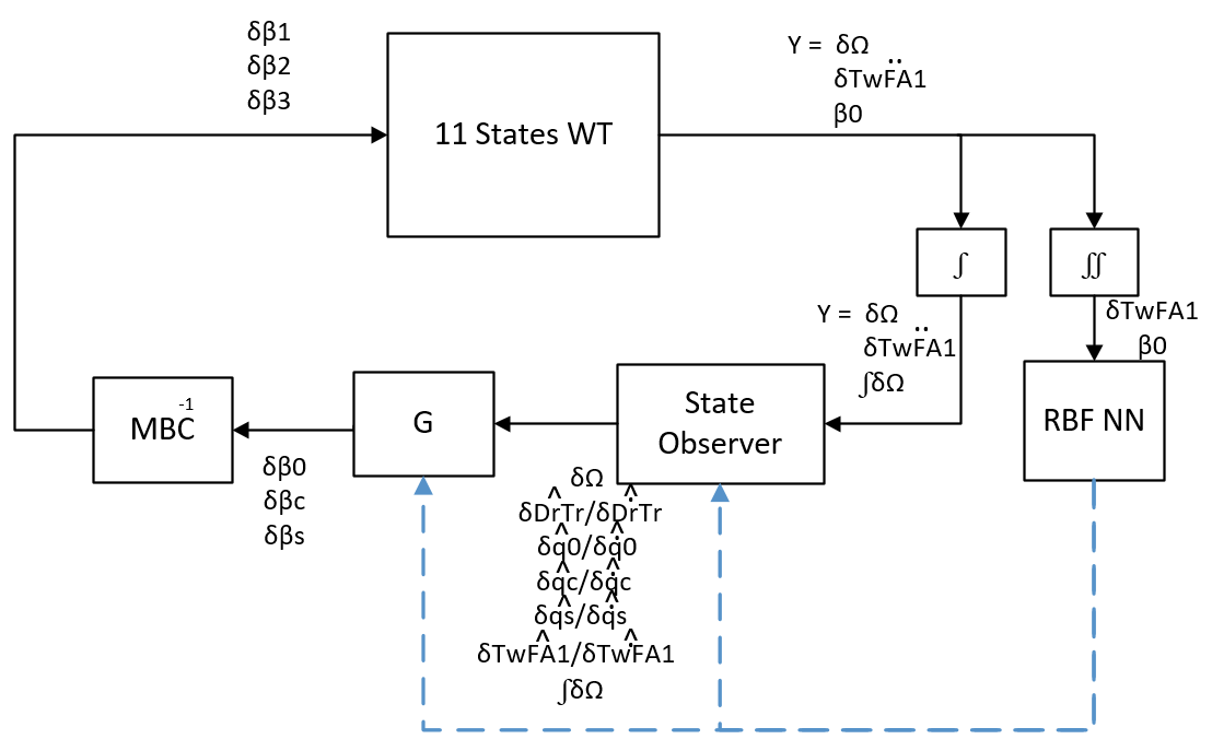
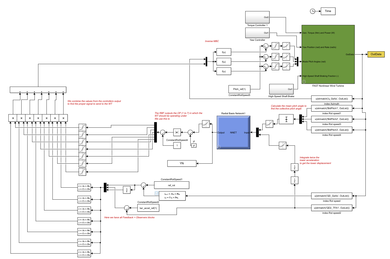
Let's start by showing you how the block diagram looks like for this type of controller:
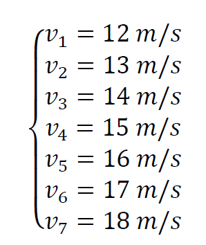
First, we linearized the WT in different OPs:
We use the same methods applied before to calculate the linearized model, reference value and gains for each of these OPs.
In order to use the gain scheduling, we need to define a parameter to be used to determine in which OP the WT is operating, we'll use the collective pitch angle (B0) and the tower displacement, because they have a direct relationship with the wind speed. By the way, the collective pitch angle can only be used as a scheduling parameter thanks to the integral term that we added to the model because it ensured the rotor speed is always on the desired value by simply increasing the collective angle. As for the tower displacement, it can be calculated from the tower acceleration.
We take the following values from the linearizations and use them as input to the RBF NN:
The outputs are gains Kbar and Gbar for each OP, but to make it easier to implement I make the output be the OP, so it ranges from 1 to 7, then the result is used to combine the output from each controller to pass it the WT. We'll see the details of this implementation later in this section.
The first step is to calculate the gains for every OP, we perform the calculations by taking all .lin files and executing the very same code we did (with a few adjustment for better resource management) for every controller before this one. You can find the script to do that on the file RBF_NN_GAINS.m under the files folder.
The second step is to train the RBF NN.
Although the training process employed here is discussed in details in Three learning phases for radial-basis-function networks, we must clarify how the training is performed using the two-phase learning technique. In the first phase, the hidden neurons’ centres or centroids (c) are calculated using the k-means technique for clustering the input data. Using the clusters’ data points, each cluster width (𝜎) is computed as the mean distance to its centre (c). The second phase is simply a linear combination of the neuron activation in the hidden layer, i.e. it takes the output from the hidden layer and linearly combine them to find the gains for achieving the target value. The script used to train the network is on the files folder.
After the training is complete, we need to intialize the weights on Matlab. The Matlab documentation explains the RBF and its implementation a bit here: Radial Basis Neural Networks
As we train the network with our own script, we need to create the RBF NN and update its weights obtained from the training. We also need to generate the Simulink model of the RBF NN. The code necessary to do that is also in the files folder. Basically, we have to assign and weights (w) and bias (b) for each layer, so that would be 4 weights we need to determine the w1, b2, w2 and b2. Please, take a look at the script on the files folder to see how this is achieve. Lastly, we need to generate the Simulink model for this model using the command:
gensim(net_pitch,DT);
Where DT is the sampling time.
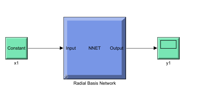
This command will open a simulink model with the RBF NN:
You can take the RBF block and use on your own model, as we'll do here.
Now that you have the model, we use it to create our own simulink model. You can find the file, along with notes to help you understand it, in the files folder as well.
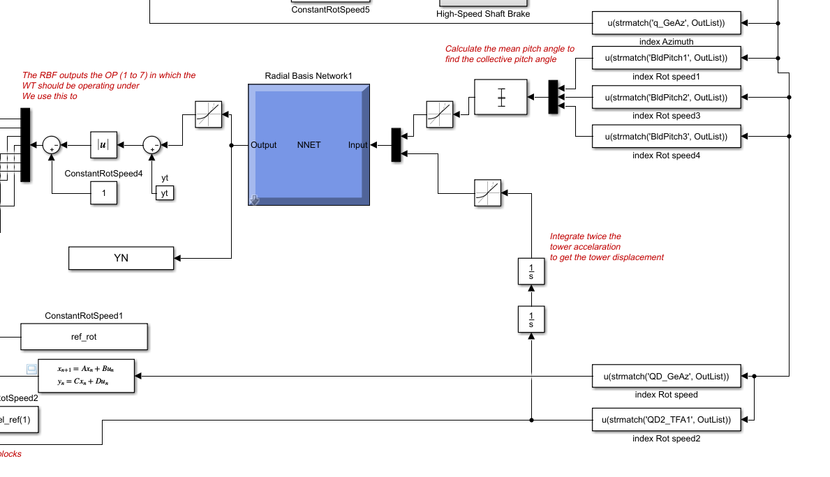
We take the RBF model and feed it with the inputs we need:
We feed the collective pitch (mean of the 3 pitchs) and the tower displacement (double integral of the tower accelaration) and it'll output the OP the WT should be on.
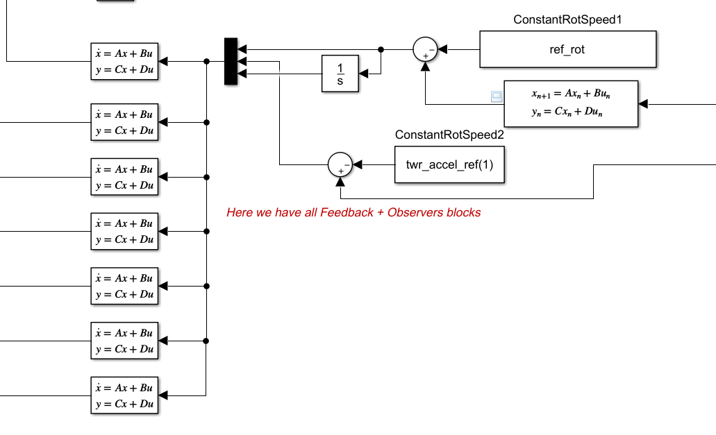
We also have to implement all the feedback controllers here to have the outputs for all OPs ready to go:
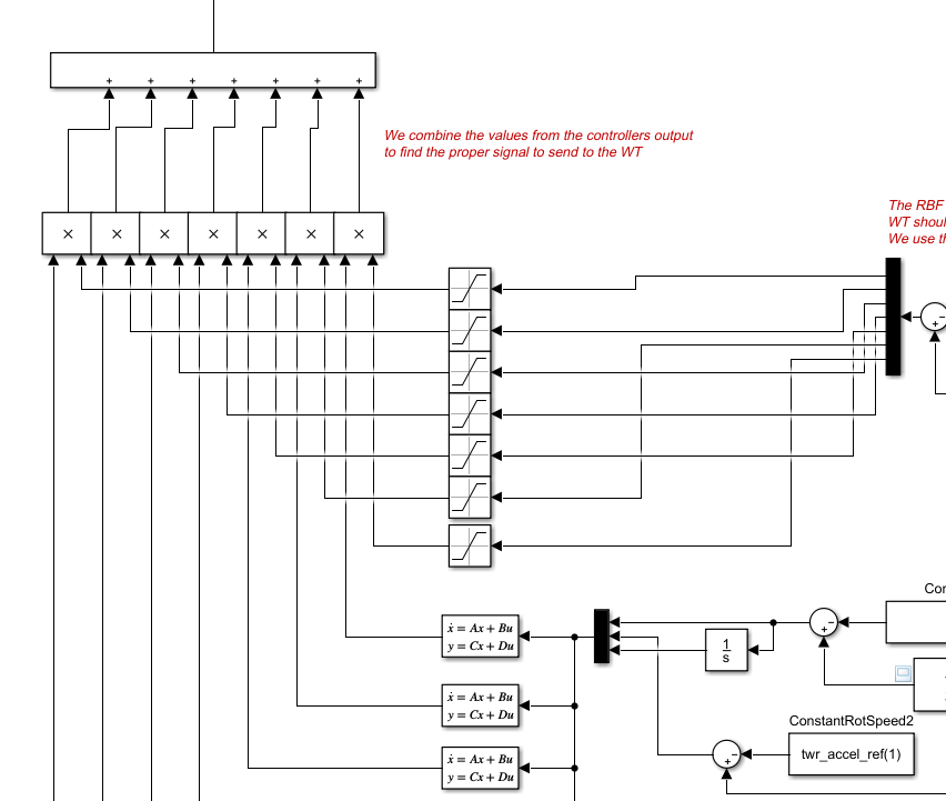
Then we combine the output from all feedback + observers according to the OP the RBF NN provided:
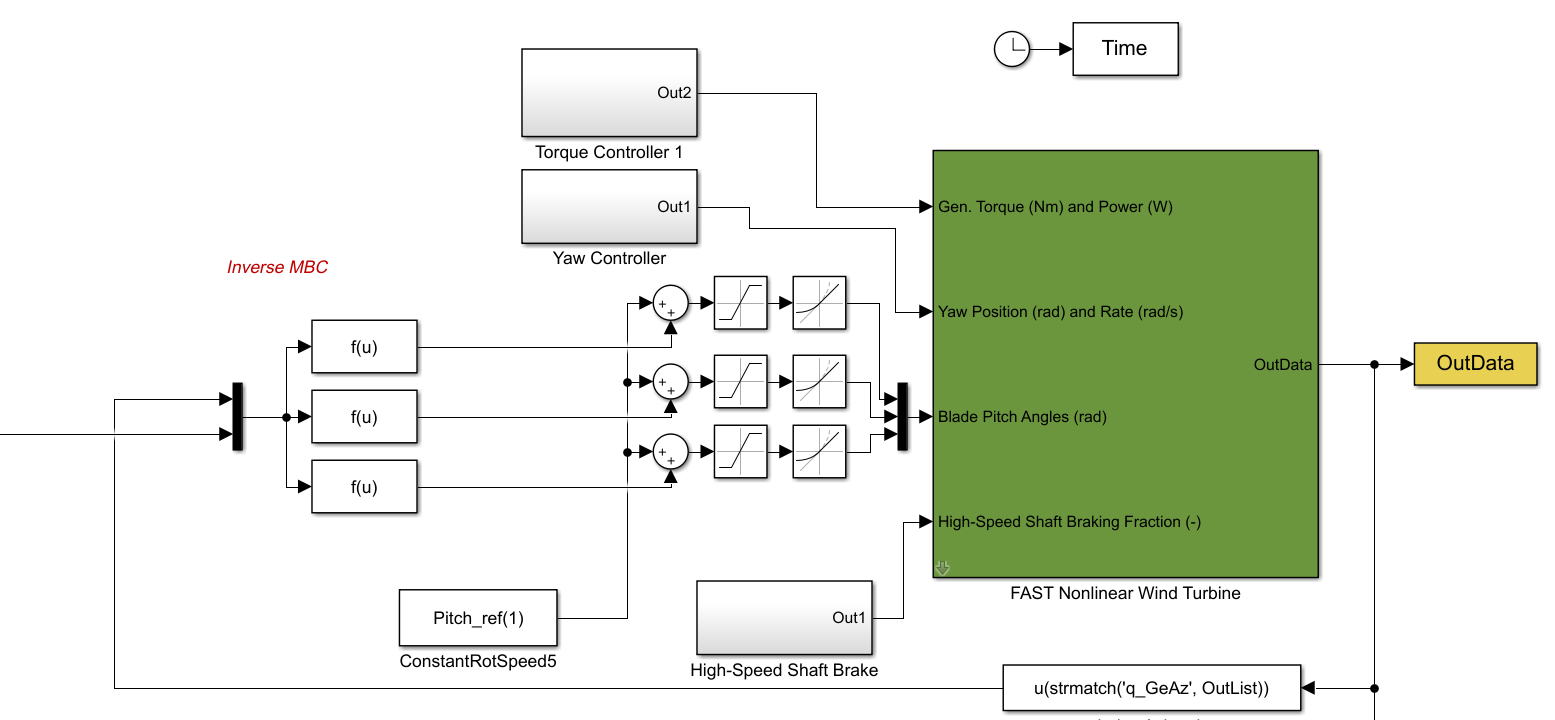
Finally, we perform the inverse MBC and send the signal to the WT:
This is the complete simulink model for this controller:
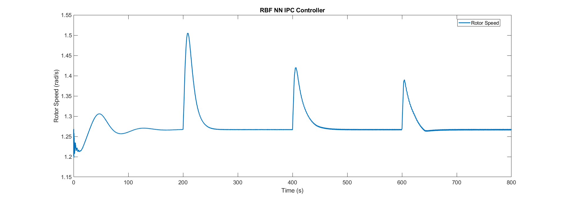
This is the rotor speed resulted from the RBF NN IPC controller we implemented:
Now, we learned how to implement a RBF NN to act as gain scheduling for different linearized system and the rotor speed is always on the set-point regardless of the wind speed.
Note that the response for the system is well damped, which will attenuate the loads on the WT components.
So far we used only constant speed winds, no turbulence what so ever, and that's rarely the case, so we need to see how this controller will perform in a more realistic scenario. We also need to compare this with the baseline PID controlller.
You can see this on the next section.
