- 原始 Markdown文档、Visio流程图、XMind思维导图见:https://github.com/LiZhengXiao99/Navigation-Learning
- 本文翻译自论文:Impact of the Earth Rotation Compensation on MEMS-IMU Preintegration of Factor Graph Optimization
- 原论文下载:http://www.i2nav.com/ueditor/jsp/upload/file/20220801/1659348408510061111.pdf
[TOC]
在基于滤波的 GNSS/INS 组合导航系统中,精密的 IMU 机械编排需要考虑到地球自转、牵连角速度、科氏加速度等的影响;然而大多数的图优化框架中的 IMU 预积分模型都没有考虑这些因素。我们提出了一种进行了地球自转补偿的滑动窗口图优化 GNSS/INS 组合导航算法,并且评估了地球自转等对 MEMS-IMU 预积分的影响。测试了 GNSS 量测缺失,采用了有效的方法对预积分结果进行评价。结果表明,此方法预积分的精度与精密机械编排的精度相当;相比之下,IMU 在不补偿地球自转的情况下,预积分的精度显著低于机械编排的精度,有显著的精度降级。当 GNSS 中断时间为 60 秒时,工业级 MEMS 的降级可能为 200% 模块,消费级 MEMS 芯片超过 10%。此外,如果 GNSS 中断时间更长,精度降级还会更显著。
在本文中,我们的目标是评估 MEMS-IMU 预积分中进行地球自转补偿的效果;利用了模拟 GNSS 中断的方法,而非 VINS 或 LINS 进行分析和评估;并且以 EKF 的 GNSS/INS 组合导航解作为 INS 精确度的基准。本论文的主要贡献如下:
- 提出了一种图优化框架下,滑动窗口 GNSS/INS 组合导航优化器,可以融合 GNSS 定位点和 IMU 预积分数据;其中我们重新定义了 IMU 预积分模型,进行了地球自转补偿。
- 采用模拟 GNSS 中断的方法来定量评估地球自转补偿对 IMU 预积分的影响,并在开阔天空地区进行三次实地测试。
- 为了充分展示地球自转补偿对不同等级 MEMS-IMU 的影响,我们采用了四个不同的 MEMS-IMU,包括一个消费级 MEMS 芯片和三个不同的工业级 MEMS 模块。
- 我们将基于因子图优化的 GNSS/INS 组合导航系统和经过改进的 IMU 预积分开源,并提供上述四个数据集。
本文各章节安排如下:下一章介绍进行地球自转补偿的 IMU 预积分模型,第三章介绍 GNSS/INS 图优化组合导航模型,第四章实验和结果中定量评估地球自转补偿对 IMU 预积分的影响,在最后做出本文的研究结论。
大多数的 IMU 预积分模型中都忽略了地球自转,例如文献 [15]、[17]、[18]、[22]、[23]、[25]–[27],这是对 IMU 精度的浪费,尤其是对于工业级或更高级的 IMU 来说。受到 IMU 精密机械编排的启发 ^[1]–[3]^,我们进一步重新定义了 IMU 预积分模型去补充地球自转 ^[24]^,在本章中将进行阐述,首先介绍 IMU 运动积分和预积分过程,然后介绍噪声传播和零偏的处理。
IMU 可以测量角速度 $\tilde{w}{\mathrm{ib}}^{\mathrm{b}}$ 和加速度 $\tilde{f}^{b}$(准确来说是比力),其中 $b$ 表示 IMU 载体坐标系($b$ 系),$i$ 表示惯性坐标系($i$ 系)。IMU 量测值受很多因素的影响,包括比例、零偏、非正交和白噪声 ^[3]^,在本论文中我们只考虑加性噪声 $n$ 和缓慢变化的零偏 $b$:
$$
\tilde{\boldsymbol{w}}{\mathrm{ib}}^{\mathrm{b}}=\boldsymbol{w}{\mathrm{ib}}^{\mathrm{b}}+\boldsymbol{b}{g}+\boldsymbol{n}{g}, \tilde{\boldsymbol{f}}^{\mathrm{b}}=\boldsymbol{f}^{\mathrm{b}}+\boldsymbol{b}{a}+\boldsymbol{n}{a},
$$
其中 $b{g}$ 和
在经典的高精度 INS 运动学模型 [1]-[3] 的基础上,我们省略了特定的微小项,得到以下简化模型:
$$
\begin{array}{l}
\dot{p}{\mathrm{wb}}^{\mathrm{w}}=\boldsymbol{v}{\mathrm{wb}}^{\mathrm{w}}, \
\dot{\boldsymbol{v}}{\mathrm{wb}}^{\mathrm{w}}=\mathbf{R}{\mathrm{b}}^{\mathrm{w}} \boldsymbol{f}^{\mathrm{b}}+\mathbf{g}^{\mathrm{w}}-2\left[\boldsymbol{w}{\mathrm{ic}}^{\mathrm{w}} \times\right] \boldsymbol{v}{\mathrm{wb}}^{\mathrm{w}}, \
\dot{\mathbf{q}}{\mathrm{b}}^{\mathrm{w}}=\frac{1}{2} \mathrm{q}{\mathrm{b}}^{\mathrm{w}} \otimes\left[\begin{array}{c}
0 \
\boldsymbol{w}{\mathrm{wb}}^{\mathrm{b}}
\end{array}\right], \boldsymbol{w}{\mathrm{wb}}^{\mathrm{b}}=\boldsymbol{w}{\mathrm{ib}}^{\mathrm{b}}-\mathbf{R}{\mathrm{w}}^{\mathrm{b}} \boldsymbol{w}{\mathrm{ic}}^{\mathrm{w}},
\end{array}
$$
其中 $w$ 表示世界坐标系($w$ 系),北东地(NED); $g^{w}$ 是 $w$ 系下的重力矢量;$e$ 表示地球坐标系($e$ 系);$w{i e}^{w}$ 是
在积分间隔
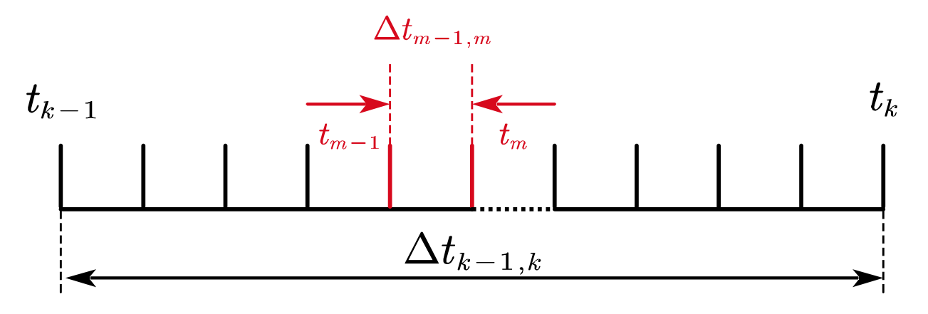
考虑到上述的运动学模型,推导出 IMU 运动积分的计算公式如下:
$$
\begin{aligned} \mathbf{q}{\mathrm{b}{m}}^{\mathrm{w}} & =\mathbf{q}{\mathrm{w}{\mathrm{i}(m-1)}}^{\mathrm{w}}\left(t_{m}\right) \otimes \mathbf{q}{\mathrm{b}{\mathrm{i}(m-1)}}^{\mathrm{w}{\mathrm{i}(m-1)}} \otimes \mathbf{q}{\mathrm{b}{m}}^{\mathrm{b}{(m-1)}} \ \boldsymbol{v}{\mathrm{wb}{m}}^{\mathrm{w}} & =\boldsymbol{v}{\mathrm{wb}{m-1}}^{\mathrm{w}}+\int_{t_{m-1}}^{t_{m}} \mathbf{R}{\mathrm{w}{\mathrm{i}(m-1)}}^{\mathrm{w}}(t) \mathbf{R}{\mathrm{b}{\mathrm{i}(m-1)}}^{\mathrm{w}{\mathrm{i}(m-1)}} \mathbf{R}{\mathrm{b}{t}}^{\mathrm{b}{\mathrm{i}(m-1)}} \boldsymbol{f}^{b} d t \ & +\int_{t_{m-1}}^{t_{m}}\left(\boldsymbol{g}^{\mathrm{w}}-2 \boldsymbol{w}{\mathrm{ie}}^{\mathrm{w}} \times \boldsymbol{v}{\mathrm{wb}{t}}^{\mathrm{w}}\right) d t \ \boldsymbol{p}{\mathrm{wb}{m}}^{\mathrm{w}} & =\boldsymbol{p}{\mathrm{wb}{m-1}}^{\mathrm{w}}+\int{t_{m-1}}^{t_{m}} \boldsymbol{v}{\mathrm{wb}{t}}^{\mathrm{w}} d t\end{aligned}
$$
其中,下标
-
P. G. Savage, “Strapdown Inertial Navigation Integration Algorithm Design Part 1: Attitude Algorithms,” J. Guid. Control Dyn., vol. 21, no. 1, pp. 19–28, 1998.
-
P. G. Savage, “Strapdown Inertial Navigation Integration Algorithm Design Part 2: Velocity and Position Algorithms,” J. Guid. Control Dyn., vol. 21, no. 2, pp. 208–221, 1998.
-
P. D. Groves, Principles of GNSS, inertial, and multisensor integrated navigation systems. Boston: Artech House, 2008.
-
C. Shen et al., “Seamless GPS/Inertial Navigation System Based on Self-Learning Square-Root Cubature Kalman Filter,” IEEE Trans. Ind. Electron., vol. 68, no. 1, pp. 499–508, 2021.
-
B. Gao, G. Hu, Y. Zhong, and X. Zhu, “Cubature Kalman Filter With Both Adaptability and Robustness for Tightly-Coupled GNSS/INS Integration,” IEEE Sens. J., vol. 21, no. 13, pp. 14997–15011, Jul. 2021.
-
Q. Zhang, X. Niu, H. Zhang, and C. Shi, “Algorithm Improvement of the Low-End GNSS/INS Systems for Land Vehicles Navigation,” Math. Probl. Eng., vol. 2013, pp. 1–12, 2013.
-
X. Niu, H. Zhang, C. Shi, K.-W. Chiang, and N. El-Sheimy, “A proposed evaluation standard for the navigation results of MEMS INS/GPS integrated systems,” in Proceedings of the International Symposium on GPS/GNSS, 2010, pp. 1–5.
-
C. Cadena et al., “Past, Present, and Future of Simultaneous Localization and Mapping: Toward the Robust-Perception Age,” IEEE Trans. Robot., vol. 32, no. 6, pp. 1309–1332, Dec. 2016.
-
G. Huang, “Visual-Inertial Navigation: A Concise Review,” in 2019 International Conference on Robotics and Automation (ICRA), May 2019, pp. 9572–9582.
-
D. Rouzaud and J. Skaloud, “Rigorous Integration of Inertial Navigation with Optical Sensors by Dynamic Networks,” Navigation, vol. 58, no. 2, pp. 141–152, Jun. 2011.
-
D. A. Cucci, M. Rehak, and J. Skaloud, “Bundle adjustment with raw inertial observations in UAV applications,” ISPRS J. Photogramm. Remote Sens., vol. 130, pp. 1–12, Aug. 2017.
-
D. A. Cucci and J. Skaloud, “ON RAW INERTIAL MEASUREMENTS IN DYNAMIC NETWORKS,” ISPRS Ann. Photogramm. Remote Sens. Spat. Inf. Sci., vol. IV-2/W5, pp. 549–557, May 2019.
-
W. Wen, T. Pfeifer, X. Bai, and L.-T. Hsu, “Factor graph optimization for GNSS/INS integration: A comparison with the extended Kalman filter,” NAVIGATION, vol. 68, no. 2, pp. 315–331, 2021.
-
S. Zhao, Y. Chen, and J. A. Farrell, “High-Precision Vehicle Navigation in Urban Environments Using an MEM’s IMU and Single-Frequency GPS Receiver,” IEEE Trans. Intell. Transp. Syst., vol. 17, no. 10, pp. 2854–2867, Oct. 2016.
-
K. Eckenhoff, P. Geneva, and G. Huang, “Closed-form preintegration methods for graph-based visual–inertial navigation,” Int. J. Robot. Res., vol. 38, no. 5, pp. 563–586, Apr. 2019.
-
W. Wen, X. Bai, Y. C. Kan, and L.-T. Hsu, “Tightly Coupled GNSS/INS Integration via Factor Graph and Aided by Fish-Eye Camera,” IEEE Trans. Veh. Technol., vol. 68, no. 11, pp. 10651–10662, Nov. 2019.
-
T. Lupton and S. Sukkarieh, “Visual-Inertial-Aided Navigation for High-Dynamic Motion in Built Environments Without Initial Conditions,” IEEE Trans. Robot., vol. 28, no. 1, pp. 61–76, Feb. 2012.
-
C. Forster, L. Carlone, F. Dellaert, and D. Scaramuzza, “On-Manifold Preintegration for Real-Time Visual--Inertial Odometry,” IEEE Trans. Robot., vol. 33, no. 1, pp. 1–21, Feb. 2017.
-
A. Barrau and S. Bonnabel, “A Mathematical Framework for IMU Error Propagation with Applications to Preintegration,” in 2020 IEEE International Conference on Robotics and Automation (ICRA), May 2020, pp. 5732–5738.
-
M. Brossard, A. Barrau, P. Chauchat, and S. Bonnabel, “Associating Uncertainty to Extended Poses for on Lie Group IMU Preintegration With Rotating Earth,” IEEE Trans. Robot., pp. 1–18, 2021.
-
Y. Luo, C. Guo, and J. Liu, “Equivariant filtering framework for inertial-integrated navigation,” Satell. Navig., vol. 2, no. 1, p. 30, Dec. 2021
-
S. Shen, N. Michael, and V. Kumar, “Tightly-coupled monocular visual-inertial fusion for autonomous flight of rotorcraft MAVs,” in 2015 IEEE International Conference on Robotics and Automation (ICRA)*, May 2015, pp. 5303–5310.
-
T. Qin, P. Li, and S. Shen, “VINS-Mono: A Robust and Versatile Monocular Visual-Inertial State Estimator,” IEEE Trans. Robot., vol. 34, no. 4, pp. 1004–1020, Aug. 2018.
-
J. Jiang, X. Niu, and J. Liu, “Improved IMU Preintegration with Gravity Change and Earth Rotation for Optimization-Based GNSS/VINS,” Remote Sens., vol. 12, no. 18, Art. no. 18, Jan. 2020.
-
L. Chang, X. Niu, and T. Liu, “GNSS/IMU/ODO/LiDAR-SLAM Integrated Navigation System Using IMU/ODO Pre-Integration,” Sensors, vol. 20, no. 17, p. 4702, Aug. 2020.
-
S. Bai, J. Lai, P. Lyu, Y. Cen, and B. Ji, “Improved Preintegration Method for GNSS/IMU/In-Vehicle Sensors Navigation using Graph Optimization,” IEEE Trans. Veh. Technol., pp. 1–1, 2021.
-
J. Henawy, Z. Li, W.-Y. Yau, and G. Seet, “Accurate IMU Factor Using
Switched Linear Systems for VIO,” IEEE Trans. Ind. Electron., vol. 68,
no. 8, pp. 7199–7208, Aug. 2021.
-
L. Wang, H. Tang, T. Zhang, Q. Chen, J. Shi, and X. Niu, “Improving the Navigation Performance of the MEMS IMU Array by Precise Calibration,” IEEE Sens. J., vol. 21, no. 22, pp. 26050–26058, 2021.
-
H. Tang, X. Niu, T. Zhang, Y. Li, and J. Liu, “OdoNet: Untethered Speed Aiding for Vehicle Navigation Without Hardware Wheeled Odometer,” IEEE Sens. J., vol. 22, no. 12, pp. 12197–12208, Jun. 2022.
-
Agarwal, Sameer, Mierle, and Keir, “Ceres Solver — A Large Scale Non-linear Optimization Library.” [Online]. Avaliable: http://ceres-solver.org/
-
J. Engel, V. Koltun, and D. Cremers, “Direct Sparse Odometry,” IEEE Trans. Pattern Anal. Mach. Intell., vol. 40, no. 3, pp. 611–625, Mar. 2018